

Feature Extraction from Hyperspectral Data Using ICA
207
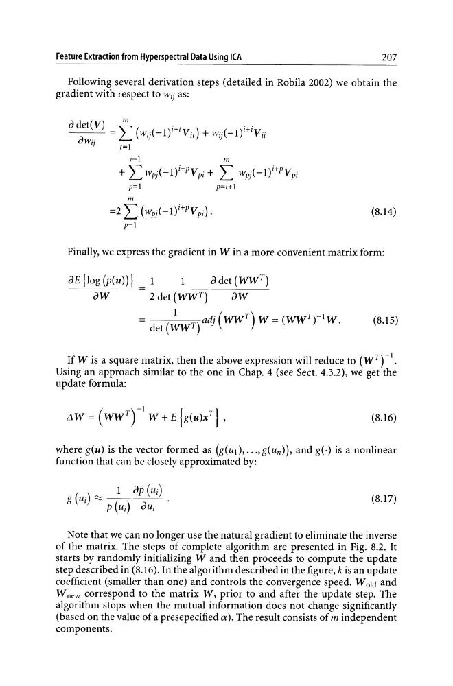
Following several derivation steps (detailed in Robila 2002) we obtain the
gradient with respect to Wij as:
~l
m
+ L wpjC_l)i+ P Vpi + L wpjC_l)i+ P Vpi
p=l
p=i+l
m
=2 L (wpj(_l)i+PVpi).
p=l
(8.14)
Finally, we express the gradient in W in a more convenient matrix form:
oE{log(p(u))} 1
1
odet(WW T )
oW
2 det (WWT)
oW
= det (~T) adj (WWT) W = (WWT)-l W.
(8.15)
If W is a square matrix, then the above expression will reduce to (wTfl.
Using an approach similar to the one in Chap. 4 (see Sect. 4.3.2), we get the
update formula:
(8.16)
where g(u) is the vector formed as (g(ud, ... ,g(un )), and g(.) is a nonlinear
function that can be closely approximated by:
(8.17)
Note that we can no longer use the natural gradient to eliminate the inverse
of the matrix. The steps of complete algorithm are presented in Fig. 8.2. It
starts by randomly initializing Wand then proceeds to compute the update
step described in (8.16). In the algorithm described in the figure, k is an update
coefficient (smaller than one) and controls the convergence speed. Wold and
W new correspond to the matrix W, prior to and after the update step. The
algorithm stops when the mutual information does not change significantly
(based on the value of a presepecified a). The result consists of m independent
components.
207
Following several derivation steps (detailed in Robila 2002) we obtain the
gradient with respect to Wij as:
~l
m
+ L wpjC_l)i+ P Vpi + L wpjC_l)i+ P Vpi
p=l
p=i+l
m
=2 L (wpj(_l)i+PVpi).
p=l
(8.14)
Finally, we express the gradient in W in a more convenient matrix form:
oE{log(p(u))} 1
1
odet(WW T )
oW
2 det (WWT)
oW
= det (~T) adj (WWT) W = (WWT)-l W.
(8.15)
If W is a square matrix, then the above expression will reduce to (wTfl.
Using an approach similar to the one in Chap. 4 (see Sect. 4.3.2), we get the
update formula:
(8.16)
where g(u) is the vector formed as (g(ud, ... ,g(un )), and g(.) is a nonlinear
function that can be closely approximated by:
(8.17)
Note that we can no longer use the natural gradient to eliminate the inverse
of the matrix. The steps of complete algorithm are presented in Fig. 8.2. It
starts by randomly initializing Wand then proceeds to compute the update
step described in (8.16). In the algorithm described in the figure, k is an update
coefficient (smaller than one) and controls the convergence speed. Wold and
W new correspond to the matrix W, prior to and after the update step. The
algorithm stops when the mutual information does not change significantly
(based on the value of a presepecified a). The result consists of m independent
components.