

Markov Random Field Models
2
1.5
0.5
o
{l.5
-1
·1 .5
-2 o
2
1.5
0.5
o
-0.5
-1
-1.5
-2 o
r -
200
400
-
200
400
600
Iteration Number
a
600
Iteration Number
b
800
800
1000
1200
1000
1200
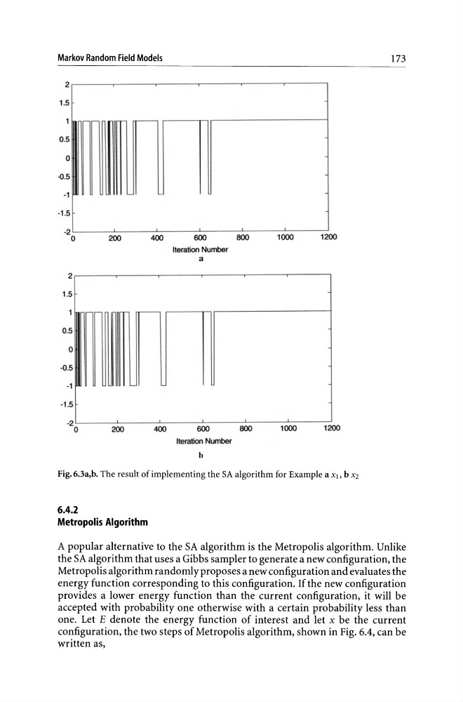
Fig.6.3a,b. The result of implementing the SA algorithm for Example a Xl, b X2
6.4.2
Metropolis Algorithm
173
A popular alternative to the SA algorithm is the Metropolis algorithm. Unlike
the SA algorithm that uses a Gibbs sampler to generate a new configuration, the
Metropolis algorithm randomly proposes a new configuration and evaluates the
energy function corresponding to this configuration. If the new configuration
provides a lower energy function than the current configuration, it will be
accepted with probability one otherwise with a certain probability less than
one. Let E denote the energy function of interest and let x be the current
configuration, the two steps of Metropolis algorithm, shown in Fig. 6.4, can be
written as,
2
1.5
0.5
o
{l.5
-1
·1 .5
-2 o
2
1.5
0.5
o
-0.5
-1
-1.5
-2 o
r -
200
400
-
200
400
600
Iteration Number
a
600
Iteration Number
b
800
800
1000
1200
1000
1200
Fig.6.3a,b. The result of implementing the SA algorithm for Example a Xl, b X2
6.4.2
Metropolis Algorithm
173
A popular alternative to the SA algorithm is the Metropolis algorithm. Unlike
the SA algorithm that uses a Gibbs sampler to generate a new configuration, the
Metropolis algorithm randomly proposes a new configuration and evaluates the
energy function corresponding to this configuration. If the new configuration
provides a lower energy function than the current configuration, it will be
accepted with probability one otherwise with a certain probability less than
one. Let E denote the energy function of interest and let x be the current
configuration, the two steps of Metropolis algorithm, shown in Fig. 6.4, can be
written as,