

172
6: Teerasit Kasetkasem
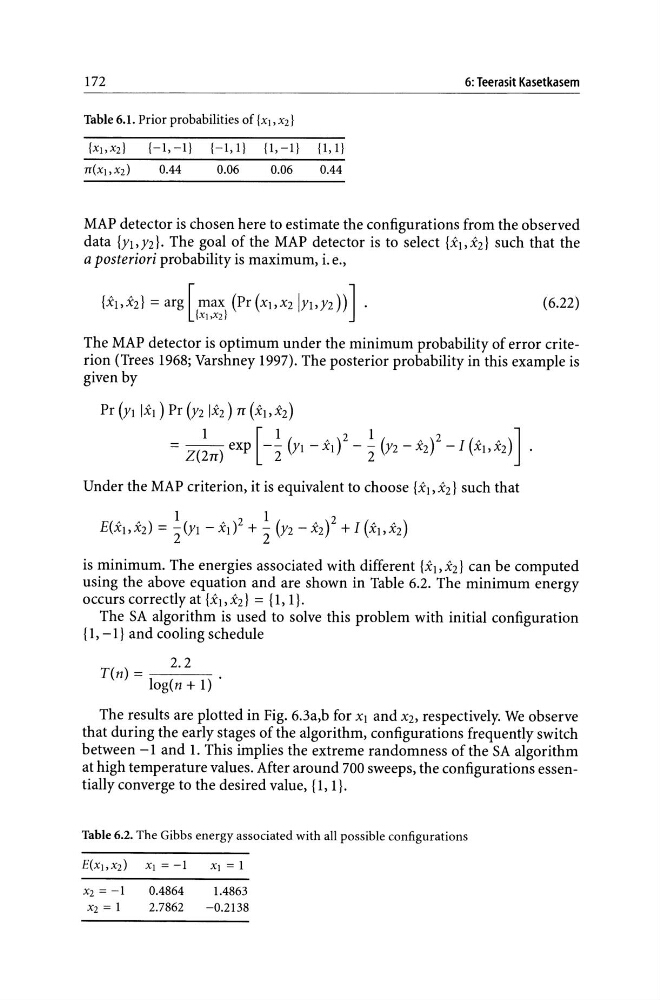
Table 6.1. Prior probabilities of {xj, Xl}
{Xj,Xl}
{-I,-I} {-I,I} {I,-I} {I,I}
n(xj, Xl)
0.44
0.06
0.06
0.44
MAP detector is chosen here to estimate the configurations from the observed
data {Yl>Y2}. The goal of the MAP detector is to select {Xl>X2} such that the
a posteriori probability is maximum, i. e.,
(6.22)
The MAP detector is optimum under the minimum probability of error criterion (Trees 1968; Varshney 1997). The posterior probability in this example is
given by
Under the MAP criterion, it is equivalent to choose {Xl> X2} such that
is minimum. The energies associated with different {XI,X2} can be computed
using the above equation and are shown in Table 6.2. The minimum energy
occurs correctly at {XI, X2} = {I, I}.
The SA algorithm is used to solve this problem with initial configuration
{ 1, -I} and cooling schedule
2.2
T ( n ) = - - -
log(n + 1)
The results are plotted in Fig. 6.3a,b for XI and X2, respectively. We observe
that during the early stages of the algorithm, configurations frequently switch
between -1 and 1. This implies the extreme randomness of the SA algorithm
at high temperature values. After around 700 sweeps, the configurations essentially converge to the desired value, {I, I}.
Table 6.2. The Gibbs energy associated with all possible configurations
Xl = -1
0.4864
1.4863
Xl = 1
2.7862
-0.2138
6: Teerasit Kasetkasem
Table 6.1. Prior probabilities of {xj, Xl}
{Xj,Xl}
{-I,-I} {-I,I} {I,-I} {I,I}
n(xj, Xl)
0.44
0.06
0.06
0.44
MAP detector is chosen here to estimate the configurations from the observed
data {Yl>Y2}. The goal of the MAP detector is to select {Xl>X2} such that the
a posteriori probability is maximum, i. e.,
(6.22)
The MAP detector is optimum under the minimum probability of error criterion (Trees 1968; Varshney 1997). The posterior probability in this example is
given by
Under the MAP criterion, it is equivalent to choose {Xl> X2} such that
is minimum. The energies associated with different {XI,X2} can be computed
using the above equation and are shown in Table 6.2. The minimum energy
occurs correctly at {XI, X2} = {I, I}.
The SA algorithm is used to solve this problem with initial configuration
{ 1, -I} and cooling schedule
2.2
T ( n ) = - - -
log(n + 1)
The results are plotted in Fig. 6.3a,b for XI and X2, respectively. We observe
that during the early stages of the algorithm, configurations frequently switch
between -1 and 1. This implies the extreme randomness of the SA algorithm
at high temperature values. After around 700 sweeps, the configurations essentially converge to the desired value, {I, I}.
Table 6.2. The Gibbs energy associated with all possible configurations
Xl = -1
0.4864
1.4863
Xl = 1
2.7862
-0.2138