

170
6: Teerasit Kasetkasem
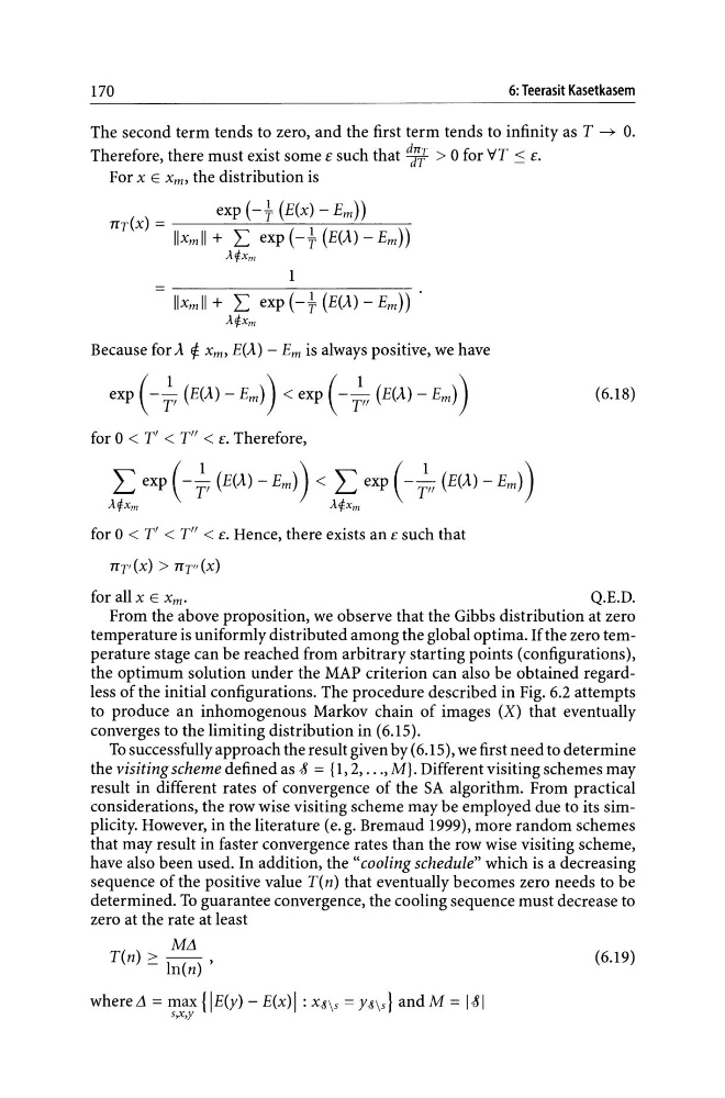
The second term tends to zero, and the first term tends to infinity as T ~ O.
Therefore, there must exist some E such that d:;.J > 0 for '1fT :::: E.
For x E X m , the distribution is
exp (-+ (E(x) - Em))
7TT(X) = -----'--'--'---::-----'-'--Ilxmll+ L exp(-+(E(A)-Em))
}."'xm
1
Ilxmll + L exp (-+ (E(A) - Em)) .
}."'xm
Because for A 1: Xm, E(A) - Em is always positive, we have
exp (- ;, (E(A) - Em)) < exp (- ;" (E(A) - Em))
(6.18)
for 0 < T' < T" < E. Therefore,
L exp (- ;, (E(A) - Em)) < L exp (- ;" (E(A) - Em))
}.~xm
}.~xm
for 0 < T' < T" < E. Hence, there exists an E such that
7TT'(X) > 7TTII(X)
for all x E X m•
Q.E.D.
From the above proposition, we observe that the Gibbs distribution at zero
temperature is uniformly distributed among the global optima. If the zero temperature stage can be reached from arbitrary starting points (configurations),
the optimum solution under the MAP criterion can also be obtained regardless of the initial configurations. The procedure described in Fig. 6.2 attempts
to produce an inhomogenous Markov chain of images (X) that eventually
converges to the limiting distribution in (6.15).
To successfully approach the result given by (6.15), we first need to determine
the visiting scheme defined as -8 = {I, 2, ... , M}. Different visiting schemes may
result in different rates of convergence of the SA algorithm. From practical
considerations, the row wise visiting scheme may be employed due to its simplicity. However, in the literature (e. g. Bremaud 1999), more random schemes
that may result in faster convergence rates than the row wise visiting scheme,
have also been used. In addition, the "cooling schedule" which is a decreasing
sequence of the positive value T(n) that eventually becomes zero needs to be
determined. To guarantee convergence, the cooling sequence must decrease to
zero at the rate at least
ML1
T(n) ;::: In(n) ,
where L1 = max {IE(y) - E(x) 1 : X-8\5 = Y8\5} and M = 1-81
5,x,y
(6.19)
6: Teerasit Kasetkasem
The second term tends to zero, and the first term tends to infinity as T ~ O.
Therefore, there must exist some E such that d:;.J > 0 for '1fT :::: E.
For x E X m , the distribution is
exp (-+ (E(x) - Em))
7TT(X) = -----'--'--'---::-----'-'--Ilxmll+ L exp(-+(E(A)-Em))
}."'xm
1
Ilxmll + L exp (-+ (E(A) - Em)) .
}."'xm
Because for A 1: Xm, E(A) - Em is always positive, we have
exp (- ;, (E(A) - Em)) < exp (- ;" (E(A) - Em))
(6.18)
for 0 < T' < T" < E. Therefore,
L exp (- ;, (E(A) - Em)) < L exp (- ;" (E(A) - Em))
}.~xm
}.~xm
for 0 < T' < T" < E. Hence, there exists an E such that
7TT'(X) > 7TTII(X)
for all x E X m•
Q.E.D.
From the above proposition, we observe that the Gibbs distribution at zero
temperature is uniformly distributed among the global optima. If the zero temperature stage can be reached from arbitrary starting points (configurations),
the optimum solution under the MAP criterion can also be obtained regardless of the initial configurations. The procedure described in Fig. 6.2 attempts
to produce an inhomogenous Markov chain of images (X) that eventually
converges to the limiting distribution in (6.15).
To successfully approach the result given by (6.15), we first need to determine
the visiting scheme defined as -8 = {I, 2, ... , M}. Different visiting schemes may
result in different rates of convergence of the SA algorithm. From practical
considerations, the row wise visiting scheme may be employed due to its simplicity. However, in the literature (e. g. Bremaud 1999), more random schemes
that may result in faster convergence rates than the row wise visiting scheme,
have also been used. In addition, the "cooling schedule" which is a decreasing
sequence of the positive value T(n) that eventually becomes zero needs to be
determined. To guarantee convergence, the cooling sequence must decrease to
zero at the rate at least
ML1
T(n) ;::: In(n) ,
where L1 = max {IE(y) - E(x) 1 : X-8\5 = Y8\5} and M = 1-81
5,x,y
(6.19)