

102
3: Hua-mei Chen
how many neighboring grid points will be involved in the joint histogram
updating procedure. For more details on B-spline functions, interested readers
are referred to Unser et al. (l993a,b).
In the GPVE scheme, the kernel functions can be of different types along
different directions. That is, we can rewrite (3.19) as
(3.20)
where fl and fz, can be different kernels. For example, if we know that the
artifacts are to appear in the y-direction only, we can choose fl as the 1st order
B-spline function but may choose fz as the 3rd order B-spline function.
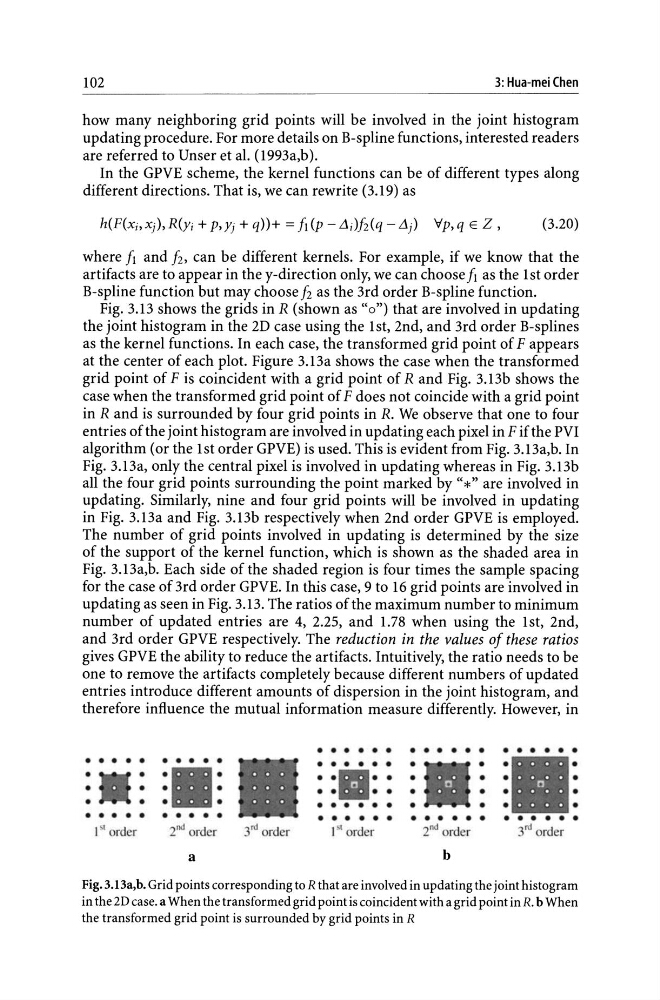
Fig. 3.13 shows the grids in R (shown as " 0") that are involved in updating
the joint histogram in the 2D case using the 1st, 2nd, and 3rd order B-splines
as the kernel functions. In each case, the transformed grid point of F appears
at the center of each plot. Figure 3.13a shows the case when the transformed
grid point of F is coincident with a grid point of R and Fig. 3.13b shows the
case when the transformed grid point of F does not coincide with a grid point
in R and is surrounded by four grid points in R. We observe that one to four
entries of the joint histogram are involved in updating each pixel in F if the PVI
algorithm (or the 1st order GPVE) is used. This is evident from Fig. 3. 13a,b. In
Fig. 3.13a, only the central pixel is involved in updating whereas in Fig. 3.13b
all the four grid points surrounding the point marked by "*" are involved in
updating. Similarly, nine and four grid points will be involved in updating
in Fig. 3.13a and Fig. 3.13b respectively when 2nd order GPVE is employed.
The number of grid points involved in updating is determined by the size
of the support of the kernel function, which is shown as the shaded area in
Fig. 3.13a,b. Each side of the shaded region is four times the sample spacing
for the case of 3rd order GPVE. In this case, 9 to 16 grid points are involved in
updating as seen in Fig. 3.13. The ratios of the maximum number to minimum
number of updated entries are 4, 2.25, and 1.78 when using the 1st, 2nd,
and 3rd order GPVE respectively. The reduction in the values of these ratios
gives GPVE the ability to reduce the artifacts. Intuitively, the ratio needs to be
one to remove the artifacts completely because different numbers of updated
entries introduce different amounts of dispersion in the joint histogram, and
therefore influence the mutual information measure differently. However, in
• • • • • • • • • • • • • • • • • •
• • • • • • • • • •
• • • • • • •
• •
•
•
•
• ••
• •
• • •
• •
•
•
• •
•
• •
• • •
• •
•
•
• •
•
• • • • • • •
• •
•
• • • • • • • • • •
• • • • • • • • • • • • • • • • • •
l SI order
2'w! order
3'd order
lSI order
2 nd order
3rd order
a
b
Fig. 3.13a,b. Grid points corresponding to R that are involved in updating the joint histogram
in the 2D case. a When the transformed grid point is coincident with a grid point in R. b When
the transformed grid point is surrounded by grid points in R
3: Hua-mei Chen
how many neighboring grid points will be involved in the joint histogram
updating procedure. For more details on B-spline functions, interested readers
are referred to Unser et al. (l993a,b).
In the GPVE scheme, the kernel functions can be of different types along
different directions. That is, we can rewrite (3.19) as
(3.20)
where fl and fz, can be different kernels. For example, if we know that the
artifacts are to appear in the y-direction only, we can choose fl as the 1st order
B-spline function but may choose fz as the 3rd order B-spline function.
Fig. 3.13 shows the grids in R (shown as " 0") that are involved in updating
the joint histogram in the 2D case using the 1st, 2nd, and 3rd order B-splines
as the kernel functions. In each case, the transformed grid point of F appears
at the center of each plot. Figure 3.13a shows the case when the transformed
grid point of F is coincident with a grid point of R and Fig. 3.13b shows the
case when the transformed grid point of F does not coincide with a grid point
in R and is surrounded by four grid points in R. We observe that one to four
entries of the joint histogram are involved in updating each pixel in F if the PVI
algorithm (or the 1st order GPVE) is used. This is evident from Fig. 3. 13a,b. In
Fig. 3.13a, only the central pixel is involved in updating whereas in Fig. 3.13b
all the four grid points surrounding the point marked by "*" are involved in
updating. Similarly, nine and four grid points will be involved in updating
in Fig. 3.13a and Fig. 3.13b respectively when 2nd order GPVE is employed.
The number of grid points involved in updating is determined by the size
of the support of the kernel function, which is shown as the shaded area in
Fig. 3.13a,b. Each side of the shaded region is four times the sample spacing
for the case of 3rd order GPVE. In this case, 9 to 16 grid points are involved in
updating as seen in Fig. 3.13. The ratios of the maximum number to minimum
number of updated entries are 4, 2.25, and 1.78 when using the 1st, 2nd,
and 3rd order GPVE respectively. The reduction in the values of these ratios
gives GPVE the ability to reduce the artifacts. Intuitively, the ratio needs to be
one to remove the artifacts completely because different numbers of updated
entries introduce different amounts of dispersion in the joint histogram, and
therefore influence the mutual information measure differently. However, in
• • • • • • • • • • • • • • • • • •
• • • • • • • • • •
• • • • • • •
• •
•
•
•
• ••
• •
• • •
• •
•
•
• •
•
• •
• • •
• •
•
•
• •
•
• • • • • • •
• •
•
• • • • • • • • • •
• • • • • • • • • • • • • • • • • •
l SI order
2'w! order
3'd order
lSI order
2 nd order
3rd order
a
b
Fig. 3.13a,b. Grid points corresponding to R that are involved in updating the joint histogram
in the 2D case. a When the transformed grid point is coincident with a grid point in R. b When
the transformed grid point is surrounded by grid points in R