

4.3 CALCULATION OF LANDSCAPE METABOLISM
A raster model implemented at a 1.5 m grid cell resolution was used to extrapolate
the SHARQ metabolic measurements across the AISA-based benthic class map. This
operation resulted in a set of maps for each mapping sensor that depicted the estimated
spatial patterns of spring-summer daytime calcification (G), daily gross photosynthesis
(P), and 24 hour respiration (R), all in units of gm C m
-2
. An excess production map
(E) (gm C m
-2
) was created for each sensor type by differencing the corresponding
estimated spatial distributions of P and R (Figure 5). The flux distributions shown on
the AISA-based reefscape metabolism maps were integrated both spatially and across
all benthic cover types to allow carbon and carbonate benthic flux estimates for the
entire study area (Figure 6).
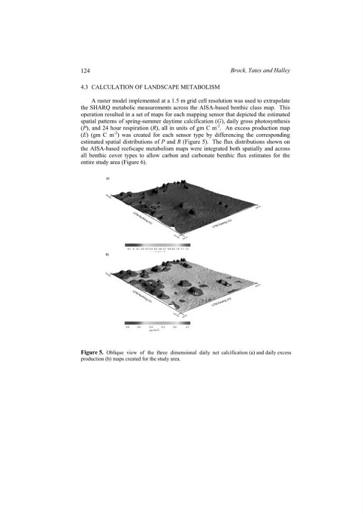
Figure 5. Oblique view of the three dimensional daily net calcification (a) and daily excess
production (b) maps created for the study area.
124
Brock, Yates and Halley
A raster model implemented at a 1.5 m grid cell resolution was used to extrapolate
the SHARQ metabolic measurements across the AISA-based benthic class map. This
operation resulted in a set of maps for each mapping sensor that depicted the estimated
spatial patterns of spring-summer daytime calcification (G), daily gross photosynthesis
(P), and 24 hour respiration (R), all in units of gm C m
-2
. An excess production map
(E) (gm C m
-2
) was created for each sensor type by differencing the corresponding
estimated spatial distributions of P and R (Figure 5). The flux distributions shown on
the AISA-based reefscape metabolism maps were integrated both spatially and across
all benthic cover types to allow carbon and carbonate benthic flux estimates for the
entire study area (Figure 6).
Figure 5. Oblique view of the three dimensional daily net calcification (a) and daily excess
production (b) maps created for the study area.
124
Brock, Yates and Halley