

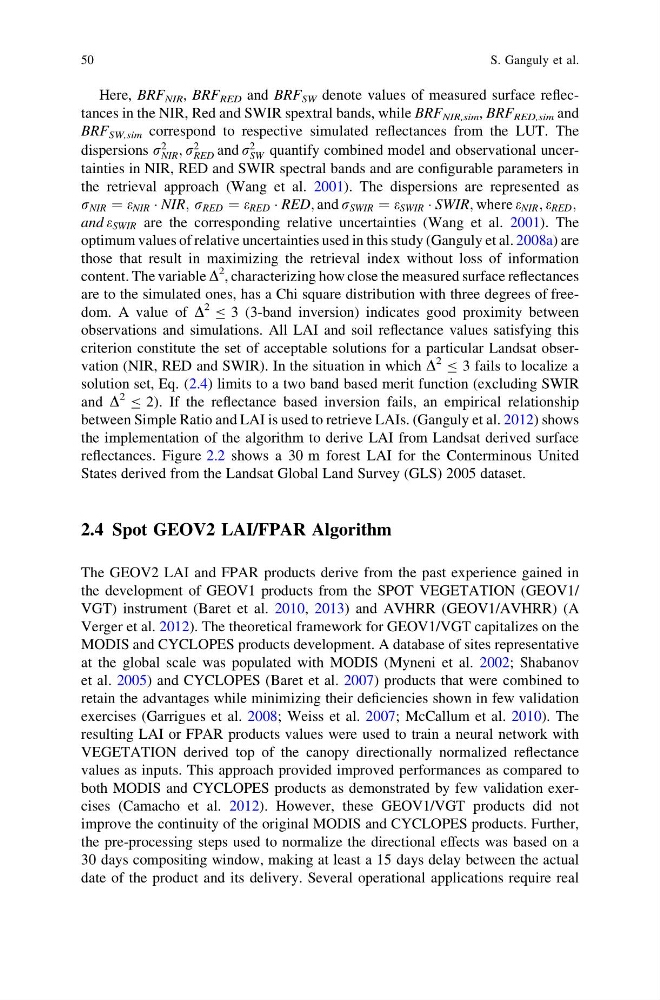
Here, BRF NIR , BRF RED and BRF SW denote values of measured surface reflectances in the NIR, Red and SWIR spextral bands, while BRF NIR,sim , BRF RED,sim and
BRF SW,sim correspond to respective simulated reflectances from the LUT. The
dispersions r
2
NIR ; r
2
RED and r
2
SW quantify combined model and observational uncertainties in NIR, RED and SWIR spectral bands and are configurable parameters in
the retrieval approach (Wang et al. 2001). The dispersions are represented as
r NIR ¼ e NIR Á NIR; r RED ¼ e RED Á RED; and r SWIR ¼ e SWIR Á SWIR; where e NIR ; e RED ;
and e SWIR are the corresponding relative uncertainties (Wang et al. 2001). The
optimum values of relative uncertainties used in this study (Ganguly et al. 2008a) are
those that result in maximizing the retrieval index without loss of information
content. The variable D
2 , characterizing how close the measured surface reflectances
are to the simulated ones, has a Chi square distribution with three degrees of freedom. A value of D
2 B 3 (3-band inversion) indicates good proximity between
observations and simulations. All LAI and soil reflectance values satisfying this
criterion constitute the set of acceptable solutions for a particular Landsat observation (NIR, RED and SWIR). In the situation in which D
2 B 3 fails to localize a
solution set, Eq. (2.4) limits to a two band based merit function (excluding SWIR
and D
2 B 2). If the reflectance based inversion fails, an empirical relationship
between Simple Ratio and LAI is used to retrieve LAIs. (Ganguly et al. 2012) shows
the implementation of the algorithm to derive LAI from Landsat derived surface
reflectances. Figure 2.2 shows a 30 m forest LAI for the Conterminous United
States derived from the Landsat Global Land Survey (GLS) 2005 dataset.
2.4 Spot GEOV2 LAI/FPAR Algorithm
The GEOV2 LAI and FPAR products derive from the past experience gained in
the development of GEOV1 products from the SPOT VEGETATION (GEOV1/
VGT) instrument (Baret et al. 2010, 2013) and AVHRR (GEOV1/AVHRR) (A
Verger et al. 2012). The theoretical framework for GEOV1/VGT capitalizes on the
MODIS and CYCLOPES products development. A database of sites representative
at the global scale was populated with MODIS (Myneni et al. 2002; Shabanov
et al. 2005) and CYCLOPES (Baret et al. 2007) products that were combined to
retain the advantages while minimizing their deficiencies shown in few validation
exercises (Garrigues et al. 2008; Weiss et al. 2007; McCallum et al. 2010). The
resulting LAI or FPAR products values were used to train a neural network with
VEGETATION derived top of the canopy directionally normalized reflectance
values as inputs. This approach provided improved performances as compared to
both MODIS and CYCLOPES products as demonstrated by few validation exercises (Camacho et al. 2012). However, these GEOV1/VGT products did not
improve the continuity of the original MODIS and CYCLOPES products. Further,
the pre-processing steps used to normalize the directional effects was based on a
30 days compositing window, making at least a 15 days delay between the actual
date of the product and its delivery. Several operational applications require real
50
S. Ganguly et al.
BRF SW,sim correspond to respective simulated reflectances from the LUT. The
dispersions r
2
NIR ; r
2
RED and r
2
SW quantify combined model and observational uncertainties in NIR, RED and SWIR spectral bands and are configurable parameters in
the retrieval approach (Wang et al. 2001). The dispersions are represented as
r NIR ¼ e NIR Á NIR; r RED ¼ e RED Á RED; and r SWIR ¼ e SWIR Á SWIR; where e NIR ; e RED ;
and e SWIR are the corresponding relative uncertainties (Wang et al. 2001). The
optimum values of relative uncertainties used in this study (Ganguly et al. 2008a) are
those that result in maximizing the retrieval index without loss of information
content. The variable D
2 , characterizing how close the measured surface reflectances
are to the simulated ones, has a Chi square distribution with three degrees of freedom. A value of D
2 B 3 (3-band inversion) indicates good proximity between
observations and simulations. All LAI and soil reflectance values satisfying this
criterion constitute the set of acceptable solutions for a particular Landsat observation (NIR, RED and SWIR). In the situation in which D
2 B 3 fails to localize a
solution set, Eq. (2.4) limits to a two band based merit function (excluding SWIR
and D
2 B 2). If the reflectance based inversion fails, an empirical relationship
between Simple Ratio and LAI is used to retrieve LAIs. (Ganguly et al. 2012) shows
the implementation of the algorithm to derive LAI from Landsat derived surface
reflectances. Figure 2.2 shows a 30 m forest LAI for the Conterminous United
States derived from the Landsat Global Land Survey (GLS) 2005 dataset.
2.4 Spot GEOV2 LAI/FPAR Algorithm
The GEOV2 LAI and FPAR products derive from the past experience gained in
the development of GEOV1 products from the SPOT VEGETATION (GEOV1/
VGT) instrument (Baret et al. 2010, 2013) and AVHRR (GEOV1/AVHRR) (A
Verger et al. 2012). The theoretical framework for GEOV1/VGT capitalizes on the
MODIS and CYCLOPES products development. A database of sites representative
at the global scale was populated with MODIS (Myneni et al. 2002; Shabanov
et al. 2005) and CYCLOPES (Baret et al. 2007) products that were combined to
retain the advantages while minimizing their deficiencies shown in few validation
exercises (Garrigues et al. 2008; Weiss et al. 2007; McCallum et al. 2010). The
resulting LAI or FPAR products values were used to train a neural network with
VEGETATION derived top of the canopy directionally normalized reflectance
values as inputs. This approach provided improved performances as compared to
both MODIS and CYCLOPES products as demonstrated by few validation exercises (Camacho et al. 2012). However, these GEOV1/VGT products did not
improve the continuity of the original MODIS and CYCLOPES products. Further,
the pre-processing steps used to normalize the directional effects was based on a
30 days compositing window, making at least a 15 days delay between the actual
date of the product and its delivery. Several operational applications require real
50
S. Ganguly et al.