

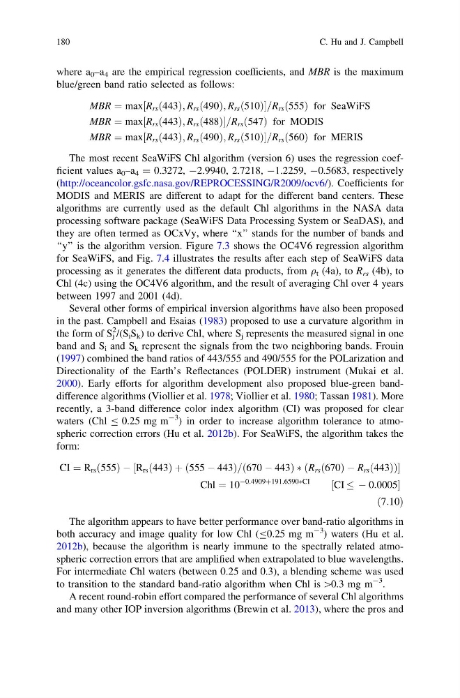
where a 0 –a 4 are the empirical regression coefficients, and MBR is the maximum
blue/green band ratio selected as follows:
MBR ¼ max R rs 443
ð
Þ; R rs 490
ð
Þ; R rs 510
ð
Þ
½
=R rs 555
ð Þ for SeaWiFS
MBR ¼ max R rs 443
ð
Þ; R rs 488
ð
Þ
½
=R rs 547
ð
Þ for MODIS
MBR ¼ max R rs 443
ð
Þ; R rs 490
ð
Þ; R rs 510
ð
Þ
½
=R rs 560
ð Þ for MERIS
The most recent SeaWiFS Chl algorithm (version 6) uses the regression coefficient values a 0 –a 4 = 0.3272, -2.9940, 2.7218, -1.2259, -0.5683, respectively
(http://oceancolor.gsfc.nasa.gov/REPROCESSING/R2009/ocv6/). Coefficients for
MODIS and MERIS are different to adapt for the different band centers. These
algorithms are currently used as the default Chl algorithms in the NASA data
processing software package (SeaWiFS Data Processing System or SeaDAS), and
they are often termed as OCxVy, where ‘‘x’’ stands for the number of bands and
‘‘y’’ is the algorithm version. Figure 7.3 shows the OC4V6 regression algorithm
for SeaWiFS, and Fig. 7.4 illustrates the results after each step of SeaWiFS data
processing as it generates the different data products, from q t (4a), to R rs (4b), to
Chl (4c) using the OC4V6 algorithm, and the result of averaging Chl over 4 years
between 1997 and 2001 (4d).
Several other forms of empirical inversion algorithms have also been proposed
in the past. Campbell and Esaias (1983) proposed to use a curvature algorithm in
the form of S j
2 /(S i S k ) to derive Chl, where S j represents the measured signal in one
band and S i and S k represent the signals from the two neighboring bands. Frouin
(1997) combined the band ratios of 443/555 and 490/555 for the POLarization and
Directionality of the Earth’s Reflectances (POLDER) instrument (Mukai et al.
2000). Early efforts for algorithm development also proposed blue-green banddifference algorithms (Viollier et al. 1978; Viollier et al. 1980; Tassan 1981). More
recently, a 3-band difference color index algorithm (CI) was proposed for clear
waters (Chl B 0.25 mg m
-3 ) in order to increase algorithm tolerance to atmospheric correction errors (Hu et al. 2012b). For SeaWiFS, the algorithm takes the
form:
CI ¼ R rs 555
ð
ÞÀ R rs 443
ð
Þþ 555 À 443
ð
Þ = 670 À 443
ð
ÞÃ R rs 670
ð
ÞÀR rs 443
ð
Þ
ð
Þ
½
Chl ¼ 10
À0:4909þ191:6590ÃCI
CI À 0:0005
½
ð7:10Þ
The algorithm appears to have better performance over band-ratio algorithms in
both accuracy and image quality for low Chl (B0.25 mg m
-3 ) waters (Hu et al.
2012b), because the algorithm is nearly immune to the spectrally related atmospheric correction errors that are amplified when extrapolated to blue wavelengths.
For intermediate Chl waters (between 0.25 and 0.3), a blending scheme was used
to transition to the standard band-ratio algorithm when Chl is [0.3 mg m
-3 .
A recent round-robin effort compared the performance of several Chl algorithms
and many other IOP inversion algorithms (Brewin et al. 2013), where the pros and
180
C. Hu and J. Campbell
blue/green band ratio selected as follows:
MBR ¼ max R rs 443
ð
Þ; R rs 490
ð
Þ; R rs 510
ð
Þ
½
=R rs 555
ð Þ for SeaWiFS
MBR ¼ max R rs 443
ð
Þ; R rs 488
ð
Þ
½
=R rs 547
ð
Þ for MODIS
MBR ¼ max R rs 443
ð
Þ; R rs 490
ð
Þ; R rs 510
ð
Þ
½
=R rs 560
ð Þ for MERIS
The most recent SeaWiFS Chl algorithm (version 6) uses the regression coefficient values a 0 –a 4 = 0.3272, -2.9940, 2.7218, -1.2259, -0.5683, respectively
(http://oceancolor.gsfc.nasa.gov/REPROCESSING/R2009/ocv6/). Coefficients for
MODIS and MERIS are different to adapt for the different band centers. These
algorithms are currently used as the default Chl algorithms in the NASA data
processing software package (SeaWiFS Data Processing System or SeaDAS), and
they are often termed as OCxVy, where ‘‘x’’ stands for the number of bands and
‘‘y’’ is the algorithm version. Figure 7.3 shows the OC4V6 regression algorithm
for SeaWiFS, and Fig. 7.4 illustrates the results after each step of SeaWiFS data
processing as it generates the different data products, from q t (4a), to R rs (4b), to
Chl (4c) using the OC4V6 algorithm, and the result of averaging Chl over 4 years
between 1997 and 2001 (4d).
Several other forms of empirical inversion algorithms have also been proposed
in the past. Campbell and Esaias (1983) proposed to use a curvature algorithm in
the form of S j
2 /(S i S k ) to derive Chl, where S j represents the measured signal in one
band and S i and S k represent the signals from the two neighboring bands. Frouin
(1997) combined the band ratios of 443/555 and 490/555 for the POLarization and
Directionality of the Earth’s Reflectances (POLDER) instrument (Mukai et al.
2000). Early efforts for algorithm development also proposed blue-green banddifference algorithms (Viollier et al. 1978; Viollier et al. 1980; Tassan 1981). More
recently, a 3-band difference color index algorithm (CI) was proposed for clear
waters (Chl B 0.25 mg m
-3 ) in order to increase algorithm tolerance to atmospheric correction errors (Hu et al. 2012b). For SeaWiFS, the algorithm takes the
form:
CI ¼ R rs 555
ð
ÞÀ R rs 443
ð
Þþ 555 À 443
ð
Þ = 670 À 443
ð
ÞÃ R rs 670
ð
ÞÀR rs 443
ð
Þ
ð
Þ
½
Chl ¼ 10
À0:4909þ191:6590ÃCI
CI À 0:0005
½
ð7:10Þ
The algorithm appears to have better performance over band-ratio algorithms in
both accuracy and image quality for low Chl (B0.25 mg m
-3 ) waters (Hu et al.
2012b), because the algorithm is nearly immune to the spectrally related atmospheric correction errors that are amplified when extrapolated to blue wavelengths.
For intermediate Chl waters (between 0.25 and 0.3), a blending scheme was used
to transition to the standard band-ratio algorithm when Chl is [0.3 mg m
-3 .
A recent round-robin effort compared the performance of several Chl algorithms
and many other IOP inversion algorithms (Brewin et al. 2013), where the pros and
180
C. Hu and J. Campbell