

When measured by a satellite above the atmosphere, R rs is modulated by the
atmospheric diffuse transmission (t), while the atmosphere itself contributes a
significant (often dominant) portion of the satellite signal (Gordon 1997). This is
expressed as:
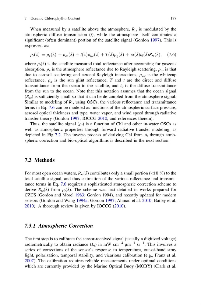
q t k
ð Þ ¼ q r k
ð Þ þ q ar k
ð Þ þ t k
ð Þq wc k
ð Þ þ T k
ð Þq g k
ð Þ þ pt k
ð Þt 0 k
ð ÞR rs k
ð Þ; ð7:6Þ
where q t (k) is the satellite measured total reflectance after accounting for gaseous
absorption, q r is the atmosphere reflectance due to Rayleigh scattering, q ar is that
due to aerosol scattering and aerosol-Rayleigh interactions, q wc is the whitecap
reflectance, q g is the sun glint reflectance, T and t are the direct and diffuse
transmittance from the ocean to the satellite, and t 0 is the diffuse transmittance
from the sun to the ocean. Note that this notation assumes that the ocean signal
(R rs ) is sufficiently small so that it can be de-coupled from the atmosphere signal.
Similar to modeling of R rs using OSCs, the various reflectance and transmittance
terms in Eq. 7.6 can be modeled as functions of the atmospheric surface pressure,
aerosol optical thickness and type, water vapor, and wind speed through radiative
transfer theory (Gordon 1997; IOCCG 2010, and references therein).
Thus, the satellite signal (q t ) is a function of Chl and other in-water OSCs as
well as atmospheric properties through forward radiative transfer modeling, as
depicted in Fig 7.2. The inverse process of deriving Chl from q t through atmospheric correction and bio-optical algorithms is described in the next section.
7.3 Methods
For most open ocean waters, R rs (k) contributes only a small portion (\10 %) to the
total satellite signal, and thus estimation of the various reflectance and transmittance terms in Eq. 7.6 requires a sophisticated atmospheric correction scheme to
derive R rs (k) from q t (k). The scheme was first detailed in works prepared for
CZCS (Gordon and Morel 1983; Gordon 1994), and recently updated for modern
sensors (Gordon and Wang 1994a; Gordon 1997; Ahmad et al. 2010; Bailey et al.
2010). A thorough review is given by IOCCG (2010).
7.3.1 Atmospheric Correction
The first step is to calibrate the sensor-received signal (usually a digitized voltage)
radiometrically to obtain radiance (L t ) in mW cm
-2 lm
-1 sr
-1 . This involves a
series of corrections of the sensor’s response to temperature, out-of-band stray
light, polarization, temporal stability, and vicarious calibration (e.g., Franz et al.
2007). The calibration requires reliable measurements under optimal conditions
which are currently provided by the Marine Optical Buoy (MOBY) (Clark et al.
7 Oceanic Chlorophyll-a Content
177
atmospheric diffuse transmission (t), while the atmosphere itself contributes a
significant (often dominant) portion of the satellite signal (Gordon 1997). This is
expressed as:
q t k
ð Þ ¼ q r k
ð Þ þ q ar k
ð Þ þ t k
ð Þq wc k
ð Þ þ T k
ð Þq g k
ð Þ þ pt k
ð Þt 0 k
ð ÞR rs k
ð Þ; ð7:6Þ
where q t (k) is the satellite measured total reflectance after accounting for gaseous
absorption, q r is the atmosphere reflectance due to Rayleigh scattering, q ar is that
due to aerosol scattering and aerosol-Rayleigh interactions, q wc is the whitecap
reflectance, q g is the sun glint reflectance, T and t are the direct and diffuse
transmittance from the ocean to the satellite, and t 0 is the diffuse transmittance
from the sun to the ocean. Note that this notation assumes that the ocean signal
(R rs ) is sufficiently small so that it can be de-coupled from the atmosphere signal.
Similar to modeling of R rs using OSCs, the various reflectance and transmittance
terms in Eq. 7.6 can be modeled as functions of the atmospheric surface pressure,
aerosol optical thickness and type, water vapor, and wind speed through radiative
transfer theory (Gordon 1997; IOCCG 2010, and references therein).
Thus, the satellite signal (q t ) is a function of Chl and other in-water OSCs as
well as atmospheric properties through forward radiative transfer modeling, as
depicted in Fig 7.2. The inverse process of deriving Chl from q t through atmospheric correction and bio-optical algorithms is described in the next section.
7.3 Methods
For most open ocean waters, R rs (k) contributes only a small portion (\10 %) to the
total satellite signal, and thus estimation of the various reflectance and transmittance terms in Eq. 7.6 requires a sophisticated atmospheric correction scheme to
derive R rs (k) from q t (k). The scheme was first detailed in works prepared for
CZCS (Gordon and Morel 1983; Gordon 1994), and recently updated for modern
sensors (Gordon and Wang 1994a; Gordon 1997; Ahmad et al. 2010; Bailey et al.
2010). A thorough review is given by IOCCG (2010).
7.3.1 Atmospheric Correction
The first step is to calibrate the sensor-received signal (usually a digitized voltage)
radiometrically to obtain radiance (L t ) in mW cm
-2 lm
-1 sr
-1 . This involves a
series of corrections of the sensor’s response to temperature, out-of-band stray
light, polarization, temporal stability, and vicarious calibration (e.g., Franz et al.
2007). The calibration requires reliable measurements under optimal conditions
which are currently provided by the Marine Optical Buoy (MOBY) (Clark et al.
7 Oceanic Chlorophyll-a Content
177