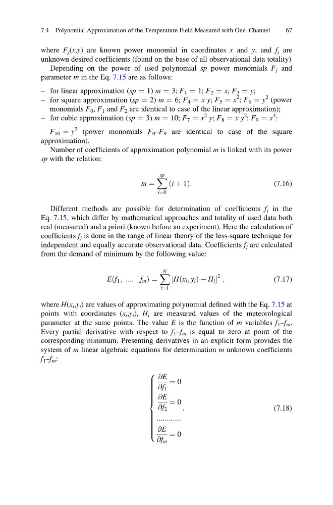
where F j (x,y) are known power monomial in coordinates x and y, and f j are
unknown desired coefficients (found on the base of all observational data totality)
Depending on the power of used polynomial sp power monomials F j and
parameter m in the Eq. 7.15 are as follows:
– for linear approximation (sp ¼ 1) m ¼ 3; F 1 ¼ 1; F 2 ¼ x; F 3 ¼ y;
– for square approximation (sp ¼ 2) m ¼ 6; F 4 ¼ x y; F 5 ¼ x
2
; F 6 ¼ y
2 (power
monomials F 0 , F 1 and F 2 are identical to case of the linear approximation);
– for cubic approximation (sp ¼ 3) m ¼ 10; F 7 ¼ x
2 y; F 8 ¼ x y
2
; F 9 ¼ x
3
:
F 10 ¼ y
3 (power monomials F 0 –F 9 are identical to case of the square
approximation).
Number of coefficients of approximation polynomial m is linked with its power
sp with the relation:
m ¼
X sp
i¼0
ði þ 1Þ:
(7.16)
Different methods are possible for determination of coefficients f j in the
Eq. 7.15, which differ by mathematical approaches and totality of used data both
real (measured) and a priori (known before an experiment). Here the calculation of
coefficients f j is done in the range of linear theory of the less-square technique for
independent and equally accurate observational data. Coefficients f j are calculated
from the demand of minimum by the following value:
Eðf 1 ; :::: ; f m Þ ¼
X N
i¼1
Hðx i ; y i Þ À H i
½
Š
2 ;
(7.17)
where H(x i ,y i ) are values of approximating polynomial defined with the Eq. 7.15 at
points with coordinates (x i ,y i ), H i are measured values of the meteorological
parameter at the same points. The value E is the function of m variables f 1 –f m .
Every partial derivative with respect to f 1 –f m is equal to zero at point of the
corresponding minimum. Presenting derivatives in an explicit form provides the
system of m linear algebraic equations for determination m unknown coefficients
f 1 –f m :
@E
@f 1
¼ 0
@E
@f 2
¼ 0
::::::::::::
@E
@f m
¼ 0
:
8
> > > > > > > > > <
> > > > > > > > > :
(7.18)
7.4 Polynomial Approximation of the Temperature Field Measured with One–Channel
67