

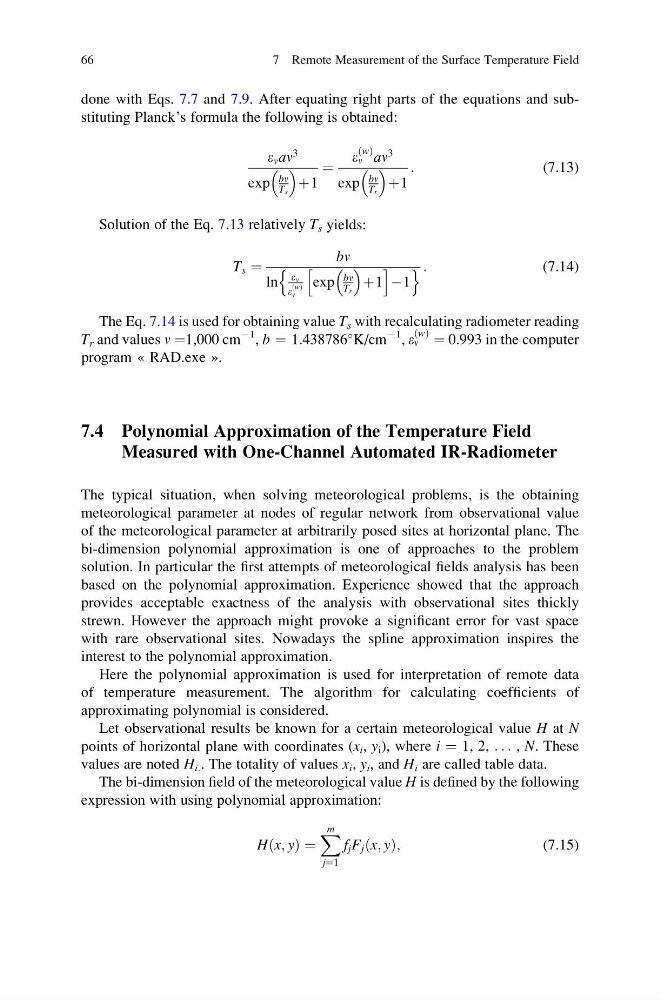
done with Eqs. 7.7 and 7.9. After equating right parts of the equations and substituting Planck’s formula the following is obtained:
e n an
3
exp
bn
Ts
þ1
¼
e
ðwÞ
n an
3
exp
bn
Tr
þ1
:
(7.13)
Solution of the Eq. 7.13 relatively T s yields:
T s ¼
bn
ln
en
e
ðwÞ
n
exp
bn
T r
þ1
h
i
À1
n
o :
(7.14)
The Eq. 7.14 is used for obtaining value T s with recalculating radiometer reading
T r and values n ¼1,000 cm
À1 , b ¼ 1.438786
K/cm
À1
, e
ðwÞ
n ¼ 0.993 in the computer
program « RAD.exe ».
7.4 Polynomial Approximation of the Temperature Field
Measured with One-Channel Automated IR-Radiometer
The typical situation, when solving meteorological problems, is the obtaining
meteorological parameter at nodes of regular network from observational value
of the meteorological parameter at arbitrarily posed sites at horizontal plane. The
bi-dimension polynomial approximation is one of approaches to the problem
solution. In particular the first attempts of meteorological fields analysis has been
based on the polynomial approximation. Experience showed that the approach
provides acceptable exactness of the analysis with observational sites thickly
strewn. However the approach might provoke a significant error for vast space
with rare observational sites. Nowadays the spline approximation inspires the
interest to the polynomial approximation.
Here the polynomial approximation is used for interpretation of remote data
of temperature measurement. The algorithm for calculating coefficients of
approximating polynomial is considered.
Let observational results be known for a certain meteorological value H at N
points of horizontal plane with coordinates (x i , y i ), where i ¼ 1, 2, . . . , N. These
values are noted H i. . The totality of values x i , y i , and H i are called table data.
The bi-dimension field of the meteorological value H is defined by the following
expression with using polynomial approximation:
Hðx; yÞ ¼
X m
j¼1
f j F j ðx; yÞ;
(7.15)
66
7 Remote Measurement of the Surface Temperature Field
e n an
3
exp
bn
Ts
þ1
¼
e
ðwÞ
n an
3
exp
bn
Tr
þ1
:
(7.13)
Solution of the Eq. 7.13 relatively T s yields:
T s ¼
bn
ln
en
e
ðwÞ
n
exp
bn
T r
þ1
h
i
À1
n
o :
(7.14)
The Eq. 7.14 is used for obtaining value T s with recalculating radiometer reading
T r and values n ¼1,000 cm
À1 , b ¼ 1.438786
K/cm
À1
, e
ðwÞ
n ¼ 0.993 in the computer
program « RAD.exe ».
7.4 Polynomial Approximation of the Temperature Field
Measured with One-Channel Automated IR-Radiometer
The typical situation, when solving meteorological problems, is the obtaining
meteorological parameter at nodes of regular network from observational value
of the meteorological parameter at arbitrarily posed sites at horizontal plane. The
bi-dimension polynomial approximation is one of approaches to the problem
solution. In particular the first attempts of meteorological fields analysis has been
based on the polynomial approximation. Experience showed that the approach
provides acceptable exactness of the analysis with observational sites thickly
strewn. However the approach might provoke a significant error for vast space
with rare observational sites. Nowadays the spline approximation inspires the
interest to the polynomial approximation.
Here the polynomial approximation is used for interpretation of remote data
of temperature measurement. The algorithm for calculating coefficients of
approximating polynomial is considered.
Let observational results be known for a certain meteorological value H at N
points of horizontal plane with coordinates (x i , y i ), where i ¼ 1, 2, . . . , N. These
values are noted H i. . The totality of values x i , y i , and H i are called table data.
The bi-dimension field of the meteorological value H is defined by the following
expression with using polynomial approximation:
Hðx; yÞ ¼
X m
j¼1
f j F j ðx; yÞ;
(7.15)
66
7 Remote Measurement of the Surface Temperature Field