

The system (7.18) might be presented in matrix form after substituting the
Eq. 7.15 to the formula (7.17), differentiating and elementary algebraic
transformations:
Df ¼ m;
(7.19)
where the (m  1)-dimensional vector f contains desired coefficients of the
approximating polynomial, the m-by-m matrix D contains only coordinates of
observational points, the (m  1)- dimensional vector m contains coordinates of
observational points with measured data. Then the problem solution might be
presented as follows:
f ¼ D
À1 m ;
(7.20)
where D
À1 is the matrix inverse of matrix D.
Thus, the calculating coefficients of approximating polynomial is reduced to
forming the matrix D and vector m on the basis of available data, Calculating the
inverse matrix D
À1
, and multiplying to the vector m.
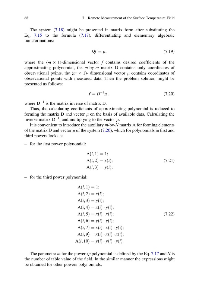
It is convenient to introduce the auxiliary m-by-N matrix A for forming elements
of the matrix D and vector m of the system (7.20), which for polynomials in first and
third powers looks as
– for the first power polynomial:
Aði; 1Þ ¼ 1;
Aði; 2Þ ¼ xðiÞ;
Aði; 3Þ ¼ yðiÞ;
(7.21)
– for the third power polynomial:
Aði; 1Þ ¼ 1;
Aði; 2Þ ¼ xðiÞ;
Aði; 3Þ ¼ yðiÞ;
Aði; 4Þ ¼ xðiÞ Á yðiÞ;
Aði; 5Þ ¼ xðiÞ Á xðiÞ;
Aði; 6Þ ¼ yðiÞ Á yðiÞ;
Aði; 7Þ ¼ xðiÞ Á xðiÞ Á yðiÞ;
Aði; 9Þ ¼ xðiÞ Á xðiÞ Á xðiÞ;
Aði; 10Þ ¼ yðiÞ Á yðiÞ Á yðiÞ:
(7.22)
The parameter m for the power sp polynomial is defined by the Eq. 7.17 and N is
the number of table value of the field. In the similar manner the expressions might
be obtained for other powers polynomials.
68
7 Remote Measurement of the Surface Temperature Field
Eq. 7.15 to the formula (7.17), differentiating and elementary algebraic
transformations:
Df ¼ m;
(7.19)
where the (m  1)-dimensional vector f contains desired coefficients of the
approximating polynomial, the m-by-m matrix D contains only coordinates of
observational points, the (m  1)- dimensional vector m contains coordinates of
observational points with measured data. Then the problem solution might be
presented as follows:
f ¼ D
À1 m ;
(7.20)
where D
À1 is the matrix inverse of matrix D.
Thus, the calculating coefficients of approximating polynomial is reduced to
forming the matrix D and vector m on the basis of available data, Calculating the
inverse matrix D
À1
, and multiplying to the vector m.
It is convenient to introduce the auxiliary m-by-N matrix A for forming elements
of the matrix D and vector m of the system (7.20), which for polynomials in first and
third powers looks as
– for the first power polynomial:
Aði; 1Þ ¼ 1;
Aði; 2Þ ¼ xðiÞ;
Aði; 3Þ ¼ yðiÞ;
(7.21)
– for the third power polynomial:
Aði; 1Þ ¼ 1;
Aði; 2Þ ¼ xðiÞ;
Aði; 3Þ ¼ yðiÞ;
Aði; 4Þ ¼ xðiÞ Á yðiÞ;
Aði; 5Þ ¼ xðiÞ Á xðiÞ;
Aði; 6Þ ¼ yðiÞ Á yðiÞ;
Aði; 7Þ ¼ xðiÞ Á xðiÞ Á yðiÞ;
Aði; 9Þ ¼ xðiÞ Á xðiÞ Á xðiÞ;
Aði; 10Þ ¼ yðiÞ Á yðiÞ Á yðiÞ:
(7.22)
The parameter m for the power sp polynomial is defined by the Eq. 7.17 and N is
the number of table value of the field. In the similar manner the expressions might
be obtained for other powers polynomials.
68
7 Remote Measurement of the Surface Temperature Field