

F
#
¼
ð
2p
0
d’
0
ð 1
0
Iðm
0
; ’
0
Þm
0 dm
0
F
"
¼ À
ð
2p
0
d’
0
ð 0
À1
Iðm
0
; ’
0
Þm
0 dm
0
(14.11)
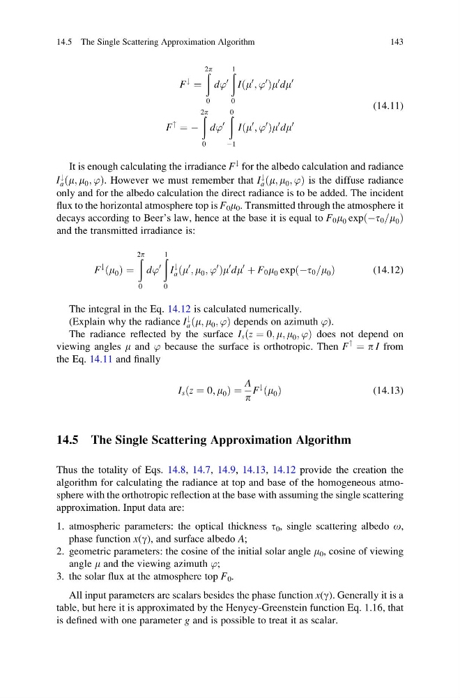
It is enough calculating the irradiance F
# for the albedo calculation and radiance
I
#
a ðm; m 0 ; ’Þ. However we must remember that I
#
a ðm; m 0 ; ’Þ is the diffuse radiance
only and for the albedo calculation the direct radiance is to be added. The incident
flux to the horizontal atmosphere top is F 0 m 0 . Transmitted through the atmosphere it
decays according to Beer’s law, hence at the base it is equal to F 0 m 0 expðÀt 0 =m 0 Þ
and the transmitted irradiance is:
F
#
ðm 0 Þ ¼
ð
2p
0
d’
0
ð 1
0
I
#
a ðm
0
; m 0 ; ’
0
Þm
0 dm
0
þ F 0 m 0 expðÀt 0 =m 0 Þ
(14.12)
The integral in the Eq. 14.12 is calculated numerically.
(Explain why the radiance I
#
a ðm; m 0 ; ’Þ depends on azimuth ’).
The radiance reflected by the surface I s ðz ¼ 0; m; m 0 ; ’Þ does not depend on
viewing angles m and ’ because the surface is orthotropic. Then F
" ¼ p I from
the Eq. 14.11 and finally
I s ðz ¼ 0; m 0 Þ ¼
A
p
F
#
ðm 0 Þ
(14.13)
14.5 The Single Scattering Approximation Algorithm
Thus the totality of Eqs. 14.8, 14.7, 14.9, 14.13, 14.12 provide the creation the
algorithm for calculating the radiance at top and base of the homogeneous atmosphere with the orthotropic reflection at the base with assuming the single scattering
approximation. Input data are:
1. atmospheric parameters: the optical thickness t 0 , single scattering albedo o,
phase function x(g), and surface albedo A;
2. geometric parameters: the cosine of the initial solar angle m 0 , cosine of viewing
angle m and the viewing azimuth ’;
3. the solar flux at the atmosphere top F 0 .
All input parameters are scalars besides the phase function x(g). Generally it is a
table, but here it is approximated by the Henyey-Greenstein function Eq. 1.16, that
is defined with one parameter g and is possible to treat it as scalar.
14.5 The Single Scattering Approximation Algorithm
143
#
¼
ð
2p
0
d’
0
ð 1
0
Iðm
0
; ’
0
Þm
0 dm
0
F
"
¼ À
ð
2p
0
d’
0
ð 0
À1
Iðm
0
; ’
0
Þm
0 dm
0
(14.11)
It is enough calculating the irradiance F
# for the albedo calculation and radiance
I
#
a ðm; m 0 ; ’Þ. However we must remember that I
#
a ðm; m 0 ; ’Þ is the diffuse radiance
only and for the albedo calculation the direct radiance is to be added. The incident
flux to the horizontal atmosphere top is F 0 m 0 . Transmitted through the atmosphere it
decays according to Beer’s law, hence at the base it is equal to F 0 m 0 expðÀt 0 =m 0 Þ
and the transmitted irradiance is:
F
#
ðm 0 Þ ¼
ð
2p
0
d’
0
ð 1
0
I
#
a ðm
0
; m 0 ; ’
0
Þm
0 dm
0
þ F 0 m 0 expðÀt 0 =m 0 Þ
(14.12)
The integral in the Eq. 14.12 is calculated numerically.
(Explain why the radiance I
#
a ðm; m 0 ; ’Þ depends on azimuth ’).
The radiance reflected by the surface I s ðz ¼ 0; m; m 0 ; ’Þ does not depend on
viewing angles m and ’ because the surface is orthotropic. Then F
" ¼ p I from
the Eq. 14.11 and finally
I s ðz ¼ 0; m 0 Þ ¼
A
p
F
#
ðm 0 Þ
(14.13)
14.5 The Single Scattering Approximation Algorithm
Thus the totality of Eqs. 14.8, 14.7, 14.9, 14.13, 14.12 provide the creation the
algorithm for calculating the radiance at top and base of the homogeneous atmosphere with the orthotropic reflection at the base with assuming the single scattering
approximation. Input data are:
1. atmospheric parameters: the optical thickness t 0 , single scattering albedo o,
phase function x(g), and surface albedo A;
2. geometric parameters: the cosine of the initial solar angle m 0 , cosine of viewing
angle m and the viewing azimuth ’;
3. the solar flux at the atmosphere top F 0 .
All input parameters are scalars besides the phase function x(g). Generally it is a
table, but here it is approximated by the Henyey-Greenstein function Eq. 1.16, that
is defined with one parameter g and is possible to treat it as scalar.
14.5 The Single Scattering Approximation Algorithm
143