

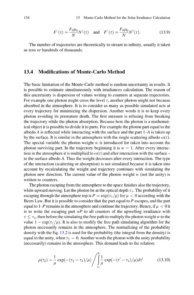
F
#
ðtÞ ¼
F 0 m 0
N
N
#
ðtÞ and F
"
ðtÞ ¼
F 0 m 0
N
N
"
ðtÞ:
(13.9)
The number of trajectories are theoretically to stream to infinity, usually it taken
as tens or hundreds of thousands.
13.4 Modifications of Monte-Carlo Method
The basic limitation of the Monte-Carlo method is random uncertainty in results. It
is possible to estimate simultaneously with irradiances calculation. The reason of
this uncertainty is dispersion of values writing to counters at separate trajectories.
For example one photon might cross the level t, another photon might not because
absorbed in the atmosphere. It is to consider as many as possible simulated acts at
every trajectory for minimizing the dispersion. Another words it is to keep every
photon avoiding its premature death. The first measure is refusing from breaking
the trajectory while the photon absorption. Because here the photon is a mathematical object it is possible to divide it to parts. For example the photon part equal to the
albedo A is reflected while interacting with the surface and the part 1–A is taken up
by the surface. It is similar in the atmosphere with the single scattering albedo o(t).
The special variable the photon weight w is introduced for taken into account the
photon surviving part. In the trajectory beginning it is w ¼ 1. After every interaction in the atmosphere it is multiplied to o(t) and after interaction with the surface –
to the surface albedo A. Thus the weight decreases after every interaction. The type
of the interaction (scattering or absorption) is not simulated because it is taken into
account by recalculating the weight and trajectory continues with simulating the
photon new direction. The current value of the photon weight w (not the unity) is
written to counters.
The photon escaping from the atmosphere to the space finishes also the trajectory,
while upward moving. Let the photon be at the optical depth t 1 . The probability of it
escaping through the atmosphere top is P ¼ expðt 1 =mÞ for m < 0 according with the
Beers Law. But it is possible to consider that the part equal to P escapes, and the part
equal to 1–P remains in the atmosphere and continue the trajectory. Hence, if m < 0 it
is to write the escaping part wP to all counters of the upwelling irradiance with
t t 1 , then before the simulating the free path to multiply the photon weight w to the
value 1 À expðt 1 =mÞ. It is also to modify the free path simulating algorithm for the
photon necessarily remains in the atmosphere. The normalizing of the probability
density with the Eq. 13.2 is used for the probability (the integral from the density) is
equal to the unity, when t 2 ¼ 0. Another words the photon with the unity probability
(necessarily) remains in the atmosphere. This demand leads to the relation:
rðt 2 Þ ¼
1
m
expðÀðt 2 À t 1 Þ=mÞ
ð 0
t 1
1
m
expðÀðt
0
À t 1 Þ=mÞdt
0
,
(13.10)
134
13 Monte-Carlo Method for the Solar Irradiance Calculation
#
ðtÞ ¼
F 0 m 0
N
N
#
ðtÞ and F
"
ðtÞ ¼
F 0 m 0
N
N
"
ðtÞ:
(13.9)
The number of trajectories are theoretically to stream to infinity, usually it taken
as tens or hundreds of thousands.
13.4 Modifications of Monte-Carlo Method
The basic limitation of the Monte-Carlo method is random uncertainty in results. It
is possible to estimate simultaneously with irradiances calculation. The reason of
this uncertainty is dispersion of values writing to counters at separate trajectories.
For example one photon might cross the level t, another photon might not because
absorbed in the atmosphere. It is to consider as many as possible simulated acts at
every trajectory for minimizing the dispersion. Another words it is to keep every
photon avoiding its premature death. The first measure is refusing from breaking
the trajectory while the photon absorption. Because here the photon is a mathematical object it is possible to divide it to parts. For example the photon part equal to the
albedo A is reflected while interacting with the surface and the part 1–A is taken up
by the surface. It is similar in the atmosphere with the single scattering albedo o(t).
The special variable the photon weight w is introduced for taken into account the
photon surviving part. In the trajectory beginning it is w ¼ 1. After every interaction in the atmosphere it is multiplied to o(t) and after interaction with the surface –
to the surface albedo A. Thus the weight decreases after every interaction. The type
of the interaction (scattering or absorption) is not simulated because it is taken into
account by recalculating the weight and trajectory continues with simulating the
photon new direction. The current value of the photon weight w (not the unity) is
written to counters.
The photon escaping from the atmosphere to the space finishes also the trajectory,
while upward moving. Let the photon be at the optical depth t 1 . The probability of it
escaping through the atmosphere top is P ¼ expðt 1 =mÞ for m < 0 according with the
Beers Law. But it is possible to consider that the part equal to P escapes, and the part
equal to 1–P remains in the atmosphere and continue the trajectory. Hence, if m < 0 it
is to write the escaping part wP to all counters of the upwelling irradiance with
t t 1 , then before the simulating the free path to multiply the photon weight w to the
value 1 À expðt 1 =mÞ. It is also to modify the free path simulating algorithm for the
photon necessarily remains in the atmosphere. The normalizing of the probability
density with the Eq. 13.2 is used for the probability (the integral from the density) is
equal to the unity, when t 2 ¼ 0. Another words the photon with the unity probability
(necessarily) remains in the atmosphere. This demand leads to the relation:
rðt 2 Þ ¼
1
m
expðÀðt 2 À t 1 Þ=mÞ
ð 0
t 1
1
m
expðÀðt
0
À t 1 Þ=mÞdt
0
,
(13.10)
134
13 Monte-Carlo Method for the Solar Irradiance Calculation