

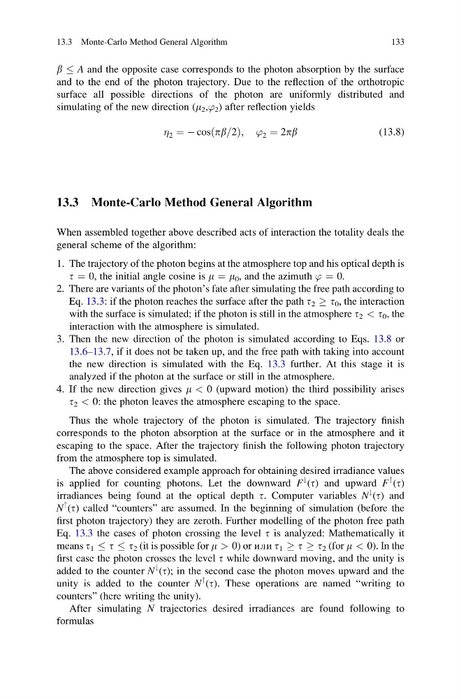
b A and the opposite case corresponds to the photon absorption by the surface
and to the end of the photon trajectory. Due to the reflection of the orthotropic
surface all possible directions of the photon are uniformly distributed and
simulating of the new direction (m 2 ,’ 2 ) after reflection yields
2 ¼ À cosðpb=2Þ; ’ 2 ¼ 2pb
(13.8)
13.3 Monte-Carlo Method General Algorithm
When assembled together above described acts of interaction the totality deals the
general scheme of the algorithm:
1. The trajectory of the photon begins at the atmosphere top and his optical depth is
t ¼ 0, the initial angle cosine is m ¼ m 0 , and the azimuth ’ ¼ 0.
2. There are variants of the photon’s fate after simulating the free path according to
Eq. 13.3: if the photon reaches the surface after the path t 2 ! t 0 , the interaction
with the surface is simulated; if the photon is still in the atmosphere t 2 < t 0 , the
interaction with the atmosphere is simulated.
3. Then the new direction of the photon is simulated according to Eqs. 13.8 or
13.6–13.7, if it does not be taken up, and the free path with taking into account
the new direction is simulated with the Eq. 13.3 further. At this stage it is
analyzed if the photon at the surface or still in the atmosphere.
4. If the new direction gives m < 0 (upward motion) the third possibility arises
t 2 < 0: the photon leaves the atmosphere escaping to the space.
Thus the whole trajectory of the photon is simulated. The trajectory finish
corresponds to the photon absorption at the surface or in the atmosphere and it
escaping to the space. After the trajectory finish the following photon trajectory
from the atmosphere top is simulated.
The above considered example approach for obtaining desired irradiance values
is applied for counting photons. Let the downward F
#
(t) and upward F
" (t)
irradiances being found at the optical depth t. Computer variables N
#
(t) and
N
" (t) called “counters” are assumed. In the beginning of simulation (before the
first photon trajectory) they are zeroth. Further modelling of the photon free path
Eq. 13.3 the cases of photon crossing the level t is analyzed: Mathematically it
means t 1 t t 2 (it is possible for m > 0) or или t 1 ! t ! t 2 (for m < 0). In the
first case the photon crosses the level t while downward moving, and the unity is
added to the counter N
#
(t); in the second case the photon moves upward and the
unity is added to the counter N
" (t). These operations are named “writing to
counters” (here writing the unity).
After simulating N trajectories desired irradiances are found following to
formulas
13.3 Monte-Carlo Method General Algorithm
133
and to the end of the photon trajectory. Due to the reflection of the orthotropic
surface all possible directions of the photon are uniformly distributed and
simulating of the new direction (m 2 ,’ 2 ) after reflection yields
2 ¼ À cosðpb=2Þ; ’ 2 ¼ 2pb
(13.8)
13.3 Monte-Carlo Method General Algorithm
When assembled together above described acts of interaction the totality deals the
general scheme of the algorithm:
1. The trajectory of the photon begins at the atmosphere top and his optical depth is
t ¼ 0, the initial angle cosine is m ¼ m 0 , and the azimuth ’ ¼ 0.
2. There are variants of the photon’s fate after simulating the free path according to
Eq. 13.3: if the photon reaches the surface after the path t 2 ! t 0 , the interaction
with the surface is simulated; if the photon is still in the atmosphere t 2 < t 0 , the
interaction with the atmosphere is simulated.
3. Then the new direction of the photon is simulated according to Eqs. 13.8 or
13.6–13.7, if it does not be taken up, and the free path with taking into account
the new direction is simulated with the Eq. 13.3 further. At this stage it is
analyzed if the photon at the surface or still in the atmosphere.
4. If the new direction gives m < 0 (upward motion) the third possibility arises
t 2 < 0: the photon leaves the atmosphere escaping to the space.
Thus the whole trajectory of the photon is simulated. The trajectory finish
corresponds to the photon absorption at the surface or in the atmosphere and it
escaping to the space. After the trajectory finish the following photon trajectory
from the atmosphere top is simulated.
The above considered example approach for obtaining desired irradiance values
is applied for counting photons. Let the downward F
#
(t) and upward F
" (t)
irradiances being found at the optical depth t. Computer variables N
#
(t) and
N
" (t) called “counters” are assumed. In the beginning of simulation (before the
first photon trajectory) they are zeroth. Further modelling of the photon free path
Eq. 13.3 the cases of photon crossing the level t is analyzed: Mathematically it
means t 1 t t 2 (it is possible for m > 0) or или t 1 ! t ! t 2 (for m < 0). In the
first case the photon crosses the level t while downward moving, and the unity is
added to the counter N
#
(t); in the second case the photon moves upward and the
unity is added to the counter N
" (t). These operations are named “writing to
counters” (here writing the unity).
After simulating N trajectories desired irradiances are found following to
formulas
13.3 Monte-Carlo Method General Algorithm
133