

method. Here the photon absorption is treated as the photon death (it is swallowed
by molecules or aerosols). The probability of the photon scattering in the atmosphere
is o 0 (t). Thus if b o 0 (t), then the photon scattering is occurring in the opposite
case the absorption is happening i.e. the end of the trajectory. Cosine of the scattering
angle w and azimuth of the scattering C are to be obtained for a new photon direction
after scattering. The phase function x(t,g) describes the probability also – it is the
probability density of scattering to the angle g. Then the Eq. 13.1 is solved for
simulating the scattering angle. The phase function is input as look-up table with
the linear interpolation that leads to the Eq. 13.1 transforming to the square equation.
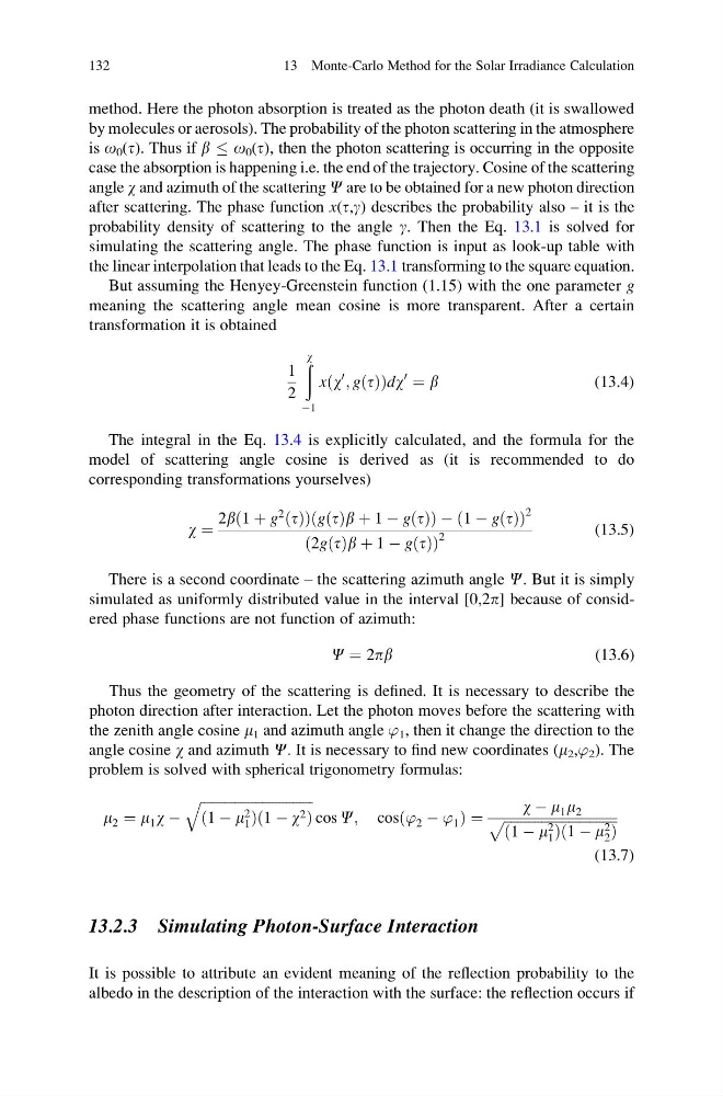
But assuming the Henyey-Greenstein function (1.15) with the one parameter g
meaning the scattering angle mean cosine is more transparent. After a certain
transformation it is obtained
1
2
ð w
À1
xðw
0
; gðtÞÞdw
0
¼ b
(13.4)
The integral in the Eq. 13.4 is explicitly calculated, and the formula for the
model of scattering angle cosine is derived as (it is recommended to do
corresponding transformations yourselves)
w ¼
2bð1 þ g
2
ðtÞÞðgðtÞb þ 1 À gðtÞÞ À ð1 À gðtÞÞ
2
ð2gðtÞb þ 1 À gðtÞÞ
2
(13.5)
There is a second coordinate – the scattering azimuth angle C. But it is simply
simulated as uniformly distributed value in the interval [0,2p] because of considered phase functions are not function of azimuth:
C ¼ 2pb
(13.6)
Thus the geometry of the scattering is defined. It is necessary to describe the
photon direction after interaction. Let the photon moves before the scattering with
the zenith angle cosine m 1 and azimuth angle ’ 1 , then it change the direction to the
angle cosine w and azimuth C. It is necessary to find new coordinates (m 2 ,’ 2 ). The
problem is solved with spherical trigonometry formulas:
m 2 ¼ m 1 w À
ffiffiffiffiffiffiffiffiffiffiffiffiffiffiffiffiffiffiffiffiffiffiffiffiffiffiffiffiffiffiffiffiffi
ð1 À m 2
1 Þð1 À w 2 Þ
q
cos C; cosð’ 2 À ’ 1 Þ ¼
w À m 1 m 2
ffiffiffiffiffiffiffiffiffiffiffiffiffiffiffiffiffiffiffiffiffiffiffiffiffiffiffiffiffiffiffiffiffi
ð1 À m 2
1 Þð1 À m 2
2 Þ
p
(13.7)
13.2.3 Simulating Photon-Surface Interaction
It is possible to attribute an evident meaning of the reflection probability to the
albedo in the description of the interaction with the surface: the reflection occurs if
132
13 Monte-Carlo Method for the Solar Irradiance Calculation
by molecules or aerosols). The probability of the photon scattering in the atmosphere
is o 0 (t). Thus if b o 0 (t), then the photon scattering is occurring in the opposite
case the absorption is happening i.e. the end of the trajectory. Cosine of the scattering
angle w and azimuth of the scattering C are to be obtained for a new photon direction
after scattering. The phase function x(t,g) describes the probability also – it is the
probability density of scattering to the angle g. Then the Eq. 13.1 is solved for
simulating the scattering angle. The phase function is input as look-up table with
the linear interpolation that leads to the Eq. 13.1 transforming to the square equation.
But assuming the Henyey-Greenstein function (1.15) with the one parameter g
meaning the scattering angle mean cosine is more transparent. After a certain
transformation it is obtained
1
2
ð w
À1
xðw
0
; gðtÞÞdw
0
¼ b
(13.4)
The integral in the Eq. 13.4 is explicitly calculated, and the formula for the
model of scattering angle cosine is derived as (it is recommended to do
corresponding transformations yourselves)
w ¼
2bð1 þ g
2
ðtÞÞðgðtÞb þ 1 À gðtÞÞ À ð1 À gðtÞÞ
2
ð2gðtÞb þ 1 À gðtÞÞ
2
(13.5)
There is a second coordinate – the scattering azimuth angle C. But it is simply
simulated as uniformly distributed value in the interval [0,2p] because of considered phase functions are not function of azimuth:
C ¼ 2pb
(13.6)
Thus the geometry of the scattering is defined. It is necessary to describe the
photon direction after interaction. Let the photon moves before the scattering with
the zenith angle cosine m 1 and azimuth angle ’ 1 , then it change the direction to the
angle cosine w and azimuth C. It is necessary to find new coordinates (m 2 ,’ 2 ). The
problem is solved with spherical trigonometry formulas:
m 2 ¼ m 1 w À
ffiffiffiffiffiffiffiffiffiffiffiffiffiffiffiffiffiffiffiffiffiffiffiffiffiffiffiffiffiffiffiffiffi
ð1 À m 2
1 Þð1 À w 2 Þ
q
cos C; cosð’ 2 À ’ 1 Þ ¼
w À m 1 m 2
ffiffiffiffiffiffiffiffiffiffiffiffiffiffiffiffiffiffiffiffiffiffiffiffiffiffiffiffiffiffiffiffiffi
ð1 À m 2
1 Þð1 À m 2
2 Þ
p
(13.7)
13.2.3 Simulating Photon-Surface Interaction
It is possible to attribute an evident meaning of the reflection probability to the
albedo in the description of the interaction with the surface: the reflection occurs if
132
13 Monte-Carlo Method for the Solar Irradiance Calculation