

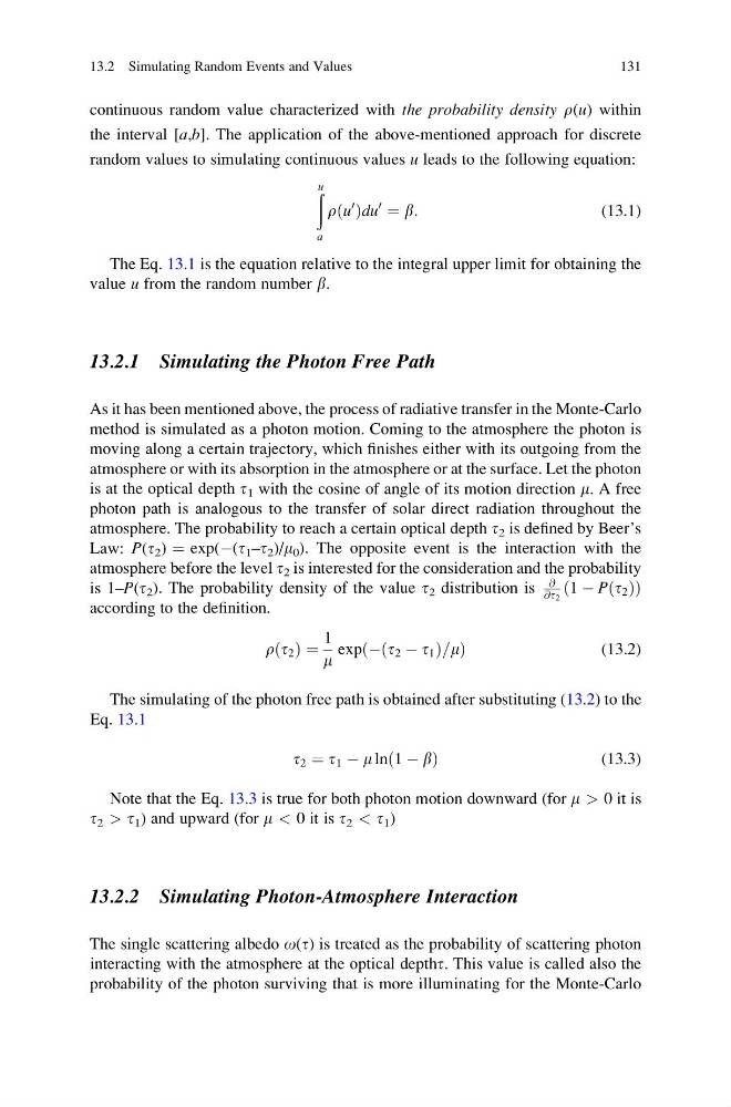
continuous random value characterized with the probability density r(u) within
the interval [a,b]. The application of the above-mentioned approach for discrete
random values to simulating continuous values u leads to the following equation:
ð u
a
rðu
0
Þdu
0
¼ b:
(13.1)
The Eq. 13.1 is the equation relative to the integral upper limit for obtaining the
value u from the random number b.
13.2.1 Simulating the Photon Free Path
As it has been mentioned above, the process of radiative transfer in the Monte-Carlo
method is simulated as a photon motion. Coming to the atmosphere the photon is
moving along a certain trajectory, which finishes either with its outgoing from the
atmosphere or with its absorption in the atmosphere or at the surface. Let the photon
is at the optical depth t 1 with the cosine of angle of its motion direction m. A free
photon path is analogous to the transfer of solar direct radiation throughout the
atmosphere. The probability to reach a certain optical depth t 2 is defined by Beer’s
Law: P(t 2 ) ¼ exp(À(t 1 –t 2 )/m 0 ). The opposite event is the interaction with the
atmosphere before the level t 2 is interested for the consideration and the probability
is 1–P(t 2 ). The probability density of the value t 2 distribution is
@
@t 2
ð1 À Pðt 2 ÞÞ
according to the definition.
rðt 2 Þ ¼
1
m
expðÀðt 2 À t 1 Þ=mÞ
(13.2)
The simulating of the photon free path is obtained after substituting (13.2) to the
Eq. 13.1
t 2 ¼ t 1 À m lnð1 À bÞ
(13.3)
Note that the Eq. 13.3 is true for both photon motion downward (for m > 0 it is
t 2 > t 1 ) and upward (for m < 0 it is t 2 < t 1 )
13.2.2 Simulating Photon-Atmosphere Interaction
The single scattering albedo o(t) is treated as the probability of scattering photon
interacting with the atmosphere at the optical deptht. This value is called also the
probability of the photon surviving that is more illuminating for the Monte-Carlo
13.2 Simulating Random Events and Values
131
the interval [a,b]. The application of the above-mentioned approach for discrete
random values to simulating continuous values u leads to the following equation:
ð u
a
rðu
0
Þdu
0
¼ b:
(13.1)
The Eq. 13.1 is the equation relative to the integral upper limit for obtaining the
value u from the random number b.
13.2.1 Simulating the Photon Free Path
As it has been mentioned above, the process of radiative transfer in the Monte-Carlo
method is simulated as a photon motion. Coming to the atmosphere the photon is
moving along a certain trajectory, which finishes either with its outgoing from the
atmosphere or with its absorption in the atmosphere or at the surface. Let the photon
is at the optical depth t 1 with the cosine of angle of its motion direction m. A free
photon path is analogous to the transfer of solar direct radiation throughout the
atmosphere. The probability to reach a certain optical depth t 2 is defined by Beer’s
Law: P(t 2 ) ¼ exp(À(t 1 –t 2 )/m 0 ). The opposite event is the interaction with the
atmosphere before the level t 2 is interested for the consideration and the probability
is 1–P(t 2 ). The probability density of the value t 2 distribution is
@
@t 2
ð1 À Pðt 2 ÞÞ
according to the definition.
rðt 2 Þ ¼
1
m
expðÀðt 2 À t 1 Þ=mÞ
(13.2)
The simulating of the photon free path is obtained after substituting (13.2) to the
Eq. 13.1
t 2 ¼ t 1 À m lnð1 À bÞ
(13.3)
Note that the Eq. 13.3 is true for both photon motion downward (for m > 0 it is
t 2 > t 1 ) and upward (for m < 0 it is t 2 < t 1 )
13.2.2 Simulating Photon-Atmosphere Interaction
The single scattering albedo o(t) is treated as the probability of scattering photon
interacting with the atmosphere at the optical deptht. This value is called also the
probability of the photon surviving that is more illuminating for the Monte-Carlo
13.2 Simulating Random Events and Values
131