

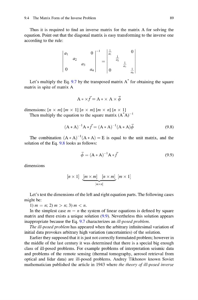
Thus it is required to find an inverse matrix for the matrix A for solving the
equation. Point out that the diagonal matrix is easy transforming to the inverse one
according to the rule:
a 1
0
a 2
a 3
0
a 4
À1
¼
1
a 1
0
1
a 2
1
a 3
0
1
a 4
Let’s multiply the Eq. 9.7 by the transposed matrix A
* for obtaining the square
matrix in spite of matrix A
A Ã Â ~ f ¼ A Ã Â A Â ~ f
dimensions: [n  m] [m  1] [n  m] [m  n] [n  1]
Then multiply the equation to the square matrix (A
*
A)
À1
ðA Ã AÞ
À1 A Ã ~ f ¼ ðA Ã AÞ
À1 A Ã A
ð
Þ ~ f
(9.8)
The combination ðA Ã AÞ
À1 A Ã A
ð
Þ¼E is equal to the unit matrix, and the
solution of the Eq. 9.8 looks as follows:
~ f ¼ A Ã A
ð
Þ
À1 A Ã ~ f
(9.9)
dimensions
n  1
½
m  m
½
n  m
½
|fflfflfflfflfflfflfflfflfflfflfflfflfflffl{zfflfflfflfflfflfflfflfflfflfflfflfflfflffl}
mÂn
½
m  1
½
Let’s test the dimensions of the left and right equation parts. The following cases
might be:
1) m ¼ n; 2) m > n; 3) m < n.
In the simplest case m ¼ n the system of linear equations is defined by square
matrix and there exists a unique solution (9.9). Nevertheless this solution appears
inappropriate because the Eq. 9.7 characterizes an ill-posed problem.
The ill-posed problem has appeared when the arbitrary infinitesimal variation of
initial data provokes arbitrary high variation (uncertainties) of the solution.
Earlier they supposed that it is just not correctly formulated problem; however in
the middle of the last century it was determined that there is a special big enough
class of ill-posed problems. For example problems of interpretation seismic data
and problems of the remote sensing (thermal tomography, aerosol retrieval from
optical and lidar data) are ill-posed problems. Andrey Tikhonov known Soviet
mathematician published the article in 1943 where the theory of ill-posed inverse
9.4 The Matrix Form of the Inverse Problem
89
equation. Point out that the diagonal matrix is easy transforming to the inverse one
according to the rule:
a 1
0
a 2
a 3
0
a 4
À1
¼
1
a 1
0
1
a 2
1
a 3
0
1
a 4
Let’s multiply the Eq. 9.7 by the transposed matrix A
* for obtaining the square
matrix in spite of matrix A
A Ã Â ~ f ¼ A Ã Â A Â ~ f
dimensions: [n  m] [m  1] [n  m] [m  n] [n  1]
Then multiply the equation to the square matrix (A
*
A)
À1
ðA Ã AÞ
À1 A Ã ~ f ¼ ðA Ã AÞ
À1 A Ã A
ð
Þ ~ f
(9.8)
The combination ðA Ã AÞ
À1 A Ã A
ð
Þ¼E is equal to the unit matrix, and the
solution of the Eq. 9.8 looks as follows:
~ f ¼ A Ã A
ð
Þ
À1 A Ã ~ f
(9.9)
dimensions
n  1
½
m  m
½
n  m
½
|fflfflfflfflfflfflfflfflfflfflfflfflfflffl{zfflfflfflfflfflfflfflfflfflfflfflfflfflffl}
mÂn
½
m  1
½
Let’s test the dimensions of the left and right equation parts. The following cases
might be:
1) m ¼ n; 2) m > n; 3) m < n.
In the simplest case m ¼ n the system of linear equations is defined by square
matrix and there exists a unique solution (9.9). Nevertheless this solution appears
inappropriate because the Eq. 9.7 characterizes an ill-posed problem.
The ill-posed problem has appeared when the arbitrary infinitesimal variation of
initial data provokes arbitrary high variation (uncertainties) of the solution.
Earlier they supposed that it is just not correctly formulated problem; however in
the middle of the last century it was determined that there is a special big enough
class of ill-posed problems. For example problems of interpretation seismic data
and problems of the remote sensing (thermal tomography, aerosol retrieval from
optical and lidar data) are ill-posed problems. Andrey Tikhonov known Soviet
mathematician published the article in 1943 where the theory of ill-posed inverse
9.4 The Matrix Form of the Inverse Problem
89