

@B
@T
T¼
TðxÞ
is the value of the Planck’s function differential over the temperature
at the point
T(x) that is possible to calculate at all levels x, with knowing the
average temperature values (average profile);
@Pnðx;top;yÞ
@x
is the known function because the CO 2 content and absorption coefficient at different spectral intervals are noted;
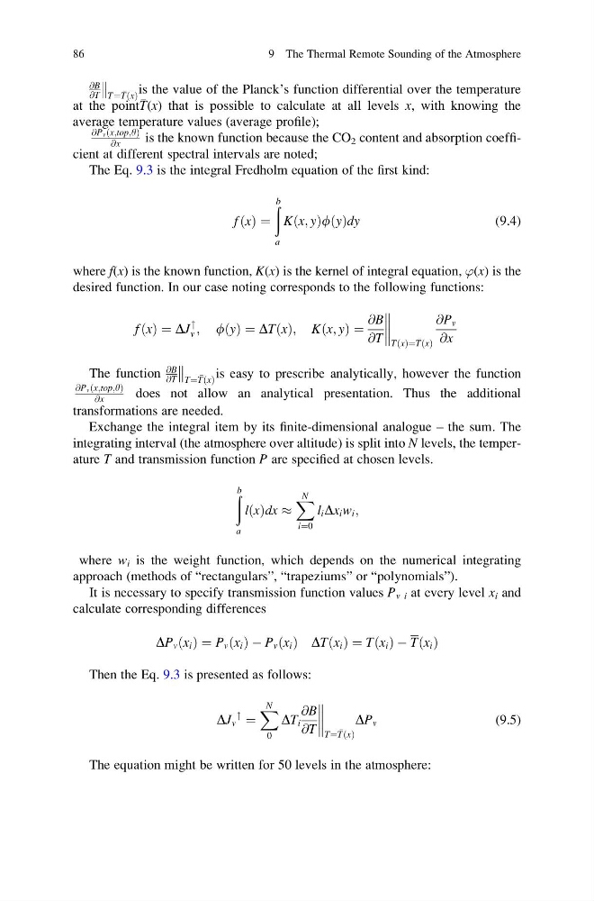
The Eq. 9.3 is the integral Fredholm equation of the first kind:
f ðxÞ ¼
ð b
a
Kðx; yÞfðyÞdy
(9.4)
where f(x) is the known function, K(x) is the kernel of integral equation, ’(x) is the
desired function. In our case noting corresponds to the following functions:
f ðxÞ ¼ DJ
"
n ; fðyÞ ¼ DTðxÞ; Kðx; yÞ ¼
@B
@T
TðxÞ¼
TðxÞ
@P n
@x
The function
@B
@T
T¼
TðxÞ
is easy to prescribe analytically, however the function
@Pnðx;top;yÞ
@x
does not allow an analytical presentation. Thus the additional
transformations are needed.
Exchange the integral item by its finite-dimensional analogue – the sum. The
integrating interval (the atmosphere over altitude) is split into N levels, the temperature T and transmission function P are specified at chosen levels.
ð b
a
lðxÞdx %
X N
i¼0
l i Dx i w i ;
where w i is the weight function, which depends on the numerical integrating
approach (methods of “rectangulars”, “trapeziums” or “polynomials”).
It is necessary to specify transmission function values P n i at every level x i and
calculate corresponding differences
DP v x i
ð Þ ¼ P v x i
ð Þ À P v x i
ð Þ DT x i
ð Þ ¼ T x i
ð Þ À T x i
ð Þ
Then the Eq. 9.3 is presented as follows:
DJ n
"
¼
X N
0
DT i
@B
@T
T¼
TðxÞ
DP n
(9.5)
The equation might be written for 50 levels in the atmosphere:
86
9 The Thermal Remote Sounding of the Atmosphere
@T
T¼
TðxÞ
is the value of the Planck’s function differential over the temperature
at the point
T(x) that is possible to calculate at all levels x, with knowing the
average temperature values (average profile);
@Pnðx;top;yÞ
@x
is the known function because the CO 2 content and absorption coefficient at different spectral intervals are noted;
The Eq. 9.3 is the integral Fredholm equation of the first kind:
f ðxÞ ¼
ð b
a
Kðx; yÞfðyÞdy
(9.4)
where f(x) is the known function, K(x) is the kernel of integral equation, ’(x) is the
desired function. In our case noting corresponds to the following functions:
f ðxÞ ¼ DJ
"
n ; fðyÞ ¼ DTðxÞ; Kðx; yÞ ¼
@B
@T
TðxÞ¼
TðxÞ
@P n
@x
The function
@B
@T
T¼
TðxÞ
is easy to prescribe analytically, however the function
@Pnðx;top;yÞ
@x
does not allow an analytical presentation. Thus the additional
transformations are needed.
Exchange the integral item by its finite-dimensional analogue – the sum. The
integrating interval (the atmosphere over altitude) is split into N levels, the temperature T and transmission function P are specified at chosen levels.
ð b
a
lðxÞdx %
X N
i¼0
l i Dx i w i ;
where w i is the weight function, which depends on the numerical integrating
approach (methods of “rectangulars”, “trapeziums” or “polynomials”).
It is necessary to specify transmission function values P n i at every level x i and
calculate corresponding differences
DP v x i
ð Þ ¼ P v x i
ð Þ À P v x i
ð Þ DT x i
ð Þ ¼ T x i
ð Þ À T x i
ð Þ
Then the Eq. 9.3 is presented as follows:
DJ n
"
¼
X N
0
DT i
@B
@T
T¼
TðxÞ
DP n
(9.5)
The equation might be written for 50 levels in the atmosphere:
86
9 The Thermal Remote Sounding of the Atmosphere