

median filter was first passed over the image. This filter reduces noise in the
classification by eliminating pixels without similar neighboring pixels. It also
diminishes the map’s original resolution from 0.5 to 1.5 m, whereby the minimum
threshold for patch size analyses was finally 2.25 m
2 . The resulting classified SSS
image was then converted to vector format by generating polygons around groups
of similar pixels. The final polygons from each class were next recorded as a single
shapefile (i.e., ArcGIS vector format), and all habitat class shapefiles were draped
over the DEM to yield a high-resolution, 3-D habitat classification map (e.g., dense
coral thicket patches in Fig. 10.13).
The workflow described above indicates that the mapped portion of the Miami
Terrace is a major cold-water coral field: the coral habitat classes (i.e., dense coral
thickets, isolated coral thickets, and coral rubble) cover approximately 76 %
(*13 km
2 ) of the site (Fig. 10.8). Coral rubble is the most abundant class (48 %),
followed by dense coral thicket (16 %), and isolated coral thicket (12 %). The
bioclastic sand dune field comprises 14 % of the mapped area, and mud-sized
sediments cover only *8 % of the site. Analyzing only ridge features, coral rubble
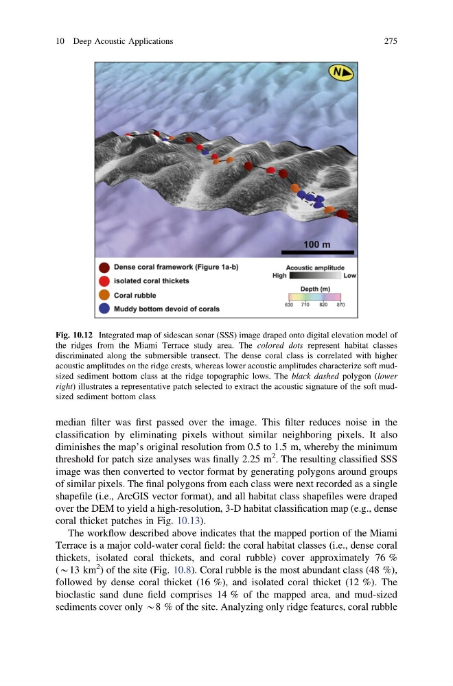
Fig. 10.12 Integrated map of sidescan sonar (SSS) image draped onto digital elevation model of
the ridges from the Miami Terrace study area. The colored dots represent habitat classes
discriminated along the submersible transect. The dense coral class is correlated with higher
acoustic amplitudes on the ridge crests, whereas lower acoustic amplitudes characterize soft mudsized sediment bottom class at the ridge topographic lows. The black dashed polygon (lower
right) illustrates a representative patch selected to extract the acoustic signature of the soft mudsized sediment bottom class
10 Deep Acoustic Applications
275
classification by eliminating pixels without similar neighboring pixels. It also
diminishes the map’s original resolution from 0.5 to 1.5 m, whereby the minimum
threshold for patch size analyses was finally 2.25 m
2 . The resulting classified SSS
image was then converted to vector format by generating polygons around groups
of similar pixels. The final polygons from each class were next recorded as a single
shapefile (i.e., ArcGIS vector format), and all habitat class shapefiles were draped
over the DEM to yield a high-resolution, 3-D habitat classification map (e.g., dense
coral thicket patches in Fig. 10.13).
The workflow described above indicates that the mapped portion of the Miami
Terrace is a major cold-water coral field: the coral habitat classes (i.e., dense coral
thickets, isolated coral thickets, and coral rubble) cover approximately 76 %
(*13 km
2 ) of the site (Fig. 10.8). Coral rubble is the most abundant class (48 %),
followed by dense coral thicket (16 %), and isolated coral thicket (12 %). The
bioclastic sand dune field comprises 14 % of the mapped area, and mud-sized
sediments cover only *8 % of the site. Analyzing only ridge features, coral rubble
Fig. 10.12 Integrated map of sidescan sonar (SSS) image draped onto digital elevation model of
the ridges from the Miami Terrace study area. The colored dots represent habitat classes
discriminated along the submersible transect. The dense coral class is correlated with higher
acoustic amplitudes on the ridge crests, whereas lower acoustic amplitudes characterize soft mudsized sediment bottom class at the ridge topographic lows. The black dashed polygon (lower
right) illustrates a representative patch selected to extract the acoustic signature of the soft mudsized sediment bottom class
10 Deep Acoustic Applications
275