

samples were generated through the stratified random sampling method
(Table 13.2). The identity of each sample was determined by the combined use of
high spatial resolution data from Google Earth, USGS 2006 National Land Cover
Data, and our field survey data. Kappa coefficients were calculated to quantify the
overall and categorical accuracies (Congalton 1991).
13.3.5 Results and Analyses
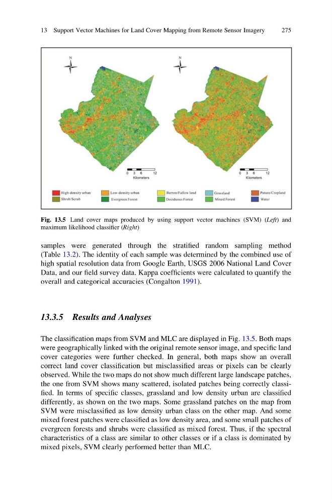
The classification maps from SVM and MLC are displayed in Fig. 13.5. Both maps
were geographically linked with the original remote sensor image, and specific land
cover categories were further checked. In general, both maps show an overall
correct land cover classification but misclassified areas or pixels can be clearly
observed. While the two maps do not show much different large landscape patches,
the one from SVM shows many scattered, isolated patches being correctly classified. In terms of specific classes, grassland and low density urban are classified
differently, as shown on the two maps. Some grassland patches on the map from
SVM were misclassified as low density urban class on the other map. And some
mixed forest patches were classified as low density area, and some small patches of
evergreen forests and shrubs were classified as mixed forest. Thus, if the spectral
characteristics of a class are similar to other classes or if a class is dominated by
mixed pixels, SVM clearly performed better than MLC.
Fig. 13.5 Land cover maps produced by using support vector machines (SVM) (Left) and
maximum likelihood classifier (Right)
13 Support Vector Machines for Land Cover Mapping from Remote Sensor Imagery
275
(Table 13.2). The identity of each sample was determined by the combined use of
high spatial resolution data from Google Earth, USGS 2006 National Land Cover
Data, and our field survey data. Kappa coefficients were calculated to quantify the
overall and categorical accuracies (Congalton 1991).
13.3.5 Results and Analyses
The classification maps from SVM and MLC are displayed in Fig. 13.5. Both maps
were geographically linked with the original remote sensor image, and specific land
cover categories were further checked. In general, both maps show an overall
correct land cover classification but misclassified areas or pixels can be clearly
observed. While the two maps do not show much different large landscape patches,
the one from SVM shows many scattered, isolated patches being correctly classified. In terms of specific classes, grassland and low density urban are classified
differently, as shown on the two maps. Some grassland patches on the map from
SVM were misclassified as low density urban class on the other map. And some
mixed forest patches were classified as low density area, and some small patches of
evergreen forests and shrubs were classified as mixed forest. Thus, if the spectral
characteristics of a class are similar to other classes or if a class is dominated by
mixed pixels, SVM clearly performed better than MLC.
Fig. 13.5 Land cover maps produced by using support vector machines (SVM) (Left) and
maximum likelihood classifier (Right)
13 Support Vector Machines for Land Cover Mapping from Remote Sensor Imagery
275