

In order to evaluate segmentation results, it is important to know accurately the
location and extent of different sea ice types. The CIS website provides daily
regional ice charts which provide a series of egg codes, indicating the sea ice
concentrations, stages of development, and form of the ice for each segment of
sea ice-covered regions. Figure 6.6 shows the daily regional ice-chart covering the
study area. By carefully interpreting the egg codes for each segment of the study
area, we found two sea ice types in Fig. 6.7, i.e. the gray ice with a thickness of 10–
15 cm and medium thick first-year ice with a thickness of 70–120 cm.
We tested different methods on three sub-images from Fig. 6.7. In this experiment we used the same parameter setting as in the experiments on synthetic image.
In order to test the log-transformation on image segmentation, we implemented a
so-called log K-Means algorithm that transforms SAR images into logarithmic
domain before performing K-Means clustering. The results are shown in
Figs. 6.8, 6.9, and 6.10.
The results on real SAR images are consistent with simulated study. And we can
extract the following conclusions based on the results. The proposed method can
accurately resist the influence of speckle noise, while in the meantime discriminate
difference sea ice types very accurately. For example, in Fig. 6.8 suggests that
KPCA can precisely delineate sea ice boundaries. Moreover, although it is challenging to identify small classes, i.e. seawater in Figs. 6.9 and 6.10, the proposed
method delineated seawater areas accurately. Another powerful model, MRF
although performed quite well in Fig. 6.9, confused seawater with certain gray
ice in Fig. 6.10.
1
0.95
0.9
0.85
0.8
0.75
0.7
9
8
7
GLCM
MRF
Prop.
Gamma Mixture
Overall Accuracy
K-Means
KPCA
6
5
4
ENL
3
2
1
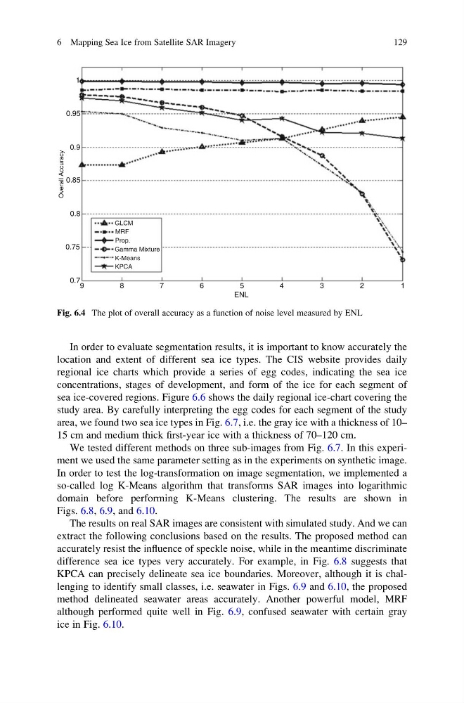
Fig. 6.4 The plot of overall accuracy as a function of noise level measured by ENL
6 Mapping Sea Ice from Satellite SAR Imagery
129
location and extent of different sea ice types. The CIS website provides daily
regional ice charts which provide a series of egg codes, indicating the sea ice
concentrations, stages of development, and form of the ice for each segment of
sea ice-covered regions. Figure 6.6 shows the daily regional ice-chart covering the
study area. By carefully interpreting the egg codes for each segment of the study
area, we found two sea ice types in Fig. 6.7, i.e. the gray ice with a thickness of 10–
15 cm and medium thick first-year ice with a thickness of 70–120 cm.
We tested different methods on three sub-images from Fig. 6.7. In this experiment we used the same parameter setting as in the experiments on synthetic image.
In order to test the log-transformation on image segmentation, we implemented a
so-called log K-Means algorithm that transforms SAR images into logarithmic
domain before performing K-Means clustering. The results are shown in
Figs. 6.8, 6.9, and 6.10.
The results on real SAR images are consistent with simulated study. And we can
extract the following conclusions based on the results. The proposed method can
accurately resist the influence of speckle noise, while in the meantime discriminate
difference sea ice types very accurately. For example, in Fig. 6.8 suggests that
KPCA can precisely delineate sea ice boundaries. Moreover, although it is challenging to identify small classes, i.e. seawater in Figs. 6.9 and 6.10, the proposed
method delineated seawater areas accurately. Another powerful model, MRF
although performed quite well in Fig. 6.9, confused seawater with certain gray
ice in Fig. 6.10.
1
0.95
0.9
0.85
0.8
0.75
0.7
9
8
7
GLCM
MRF
Prop.
Gamma Mixture
Overall Accuracy
K-Means
KPCA
6
5
4
ENL
3
2
1
Fig. 6.4 The plot of overall accuracy as a function of noise level measured by ENL
6 Mapping Sea Ice from Satellite SAR Imagery
129