

302
Alminas ˇ
Civilis, Christian S. Jensen, and Stardas Pakalnis
Algorithm PPSA(mopa, t)
1. m pred ← mopa.m
2. v pred ← mopa.plspd
3. t pred ← t − mopa.t
4. while t pred > 0 do
5. accel ← getAcceleration (m pred , mopa.apf )
6. S ← accel.end − m pred
7. dt ← 0
8. if v
2
pred + 2 · accel.a · S ≥ 0 ∧ accel.a 0 then
9.
dt 1 ←
− v pred +
v
2
pred + 2 · accel.a · S
/accel.a
10.
dt 2 ←
− v pred −
v
2
pred + 2 · accel.a · S
/accel.a
11.
dt ← max
0, min({dt|dt ∈ {dt 1 , dt 2 } ∧ dt > 0})
12. if dt = 0 then dt ← S /v pred
13.
accel.a ← 0
14. if t pred < dt then dt ← t pred
15. m pred ← m pred + v pred · dt + accel.a · dt
2
/2
16. v pred ← v pred + accel.a · dt
17. t pred ← t pred − dt
18. if m pred ≥ Mmopa.pl, mopa.pl.p end ) then return mopa.pl.p end
19. return M
−1 (mopa.pl, m pred )
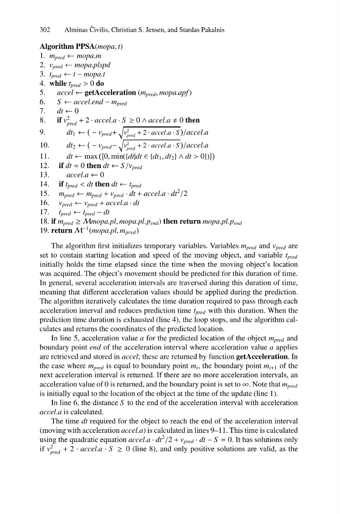
The algorithm first initializes temporary variables. Variables m pred and v pred are
set to contain starting location and speed of the moving object, and variable t pred
initially holds the time elapsed since the time when the moving object’s location
was acquired. The object’s movement should be predicted for this duration of time.
In general, several acceleration intervals are traversed during this duration of time,
meaning that different acceleration values should be applied during the prediction.
The algorithm iteratively calculates the time duration required to pass through each
acceleration interval and reduces prediction time t pred with this duration. When the
prediction time duration is exhausted (line 4), the loop stops, and the algorithm calculates and returns the coordinates of the predicted location.
In line 5, acceleration value a for the predicted location of the object m pred and
boundary point end of the acceleration interval where acceleration value a applies
are retrieved and stored in accel; these are returned by function getAcceleration. In
the case where m pred is equal to boundary point m i , the boundary point m i+1 of the
next acceleration interval is returned. If there are no more acceleration intervals, an
acceleration value of 0 is returned, and the boundary point is set to ∞. Note that m pred
is initially equal to the location of the object at the time of the update (line 1).
In line 6, the distance S to the end of the acceleration interval with acceleration
accel.a is calculated.
The time dt required for the object to reach the end of the acceleration interval
(moving with acceleration accel.a) is calculated in lines 9–11. This time is calculated
using the quadratic equation accel.a · dt
2
/2 + v pred · dt − S = 0. It has solutions only
if v
2
pred + 2 · accel.a · S ≥ 0 (line 8), and only positive solutions are valid, as the
Alminas ˇ
Civilis, Christian S. Jensen, and Stardas Pakalnis
Algorithm PPSA(mopa, t)
1. m pred ← mopa.m
2. v pred ← mopa.plspd
3. t pred ← t − mopa.t
4. while t pred > 0 do
5. accel ← getAcceleration (m pred , mopa.apf )
6. S ← accel.end − m pred
7. dt ← 0
8. if v
2
pred + 2 · accel.a · S ≥ 0 ∧ accel.a 0 then
9.
dt 1 ←
− v pred +
v
2
pred + 2 · accel.a · S
/accel.a
10.
dt 2 ←
− v pred −
v
2
pred + 2 · accel.a · S
/accel.a
11.
dt ← max
0, min({dt|dt ∈ {dt 1 , dt 2 } ∧ dt > 0})
12. if dt = 0 then dt ← S /v pred
13.
accel.a ← 0
14. if t pred < dt then dt ← t pred
15. m pred ← m pred + v pred · dt + accel.a · dt
2
/2
16. v pred ← v pred + accel.a · dt
17. t pred ← t pred − dt
18. if m pred ≥ Mmopa.pl, mopa.pl.p end ) then return mopa.pl.p end
19. return M
−1 (mopa.pl, m pred )
The algorithm first initializes temporary variables. Variables m pred and v pred are
set to contain starting location and speed of the moving object, and variable t pred
initially holds the time elapsed since the time when the moving object’s location
was acquired. The object’s movement should be predicted for this duration of time.
In general, several acceleration intervals are traversed during this duration of time,
meaning that different acceleration values should be applied during the prediction.
The algorithm iteratively calculates the time duration required to pass through each
acceleration interval and reduces prediction time t pred with this duration. When the
prediction time duration is exhausted (line 4), the loop stops, and the algorithm calculates and returns the coordinates of the predicted location.
In line 5, acceleration value a for the predicted location of the object m pred and
boundary point end of the acceleration interval where acceleration value a applies
are retrieved and stored in accel; these are returned by function getAcceleration. In
the case where m pred is equal to boundary point m i , the boundary point m i+1 of the
next acceleration interval is returned. If there are no more acceleration intervals, an
acceleration value of 0 is returned, and the boundary point is set to ∞. Note that m pred
is initially equal to the location of the object at the time of the update (line 1).
In line 6, the distance S to the end of the acceleration interval with acceleration
accel.a is calculated.
The time dt required for the object to reach the end of the acceleration interval
(moving with acceleration accel.a) is calculated in lines 9–11. This time is calculated
using the quadratic equation accel.a · dt
2
/2 + v pred · dt − S = 0. It has solutions only
if v
2
pred + 2 · accel.a · S ≥ 0 (line 8), and only positive solutions are valid, as the