

13 Tracking of Moving Objects with Accuracy Guarantees
299
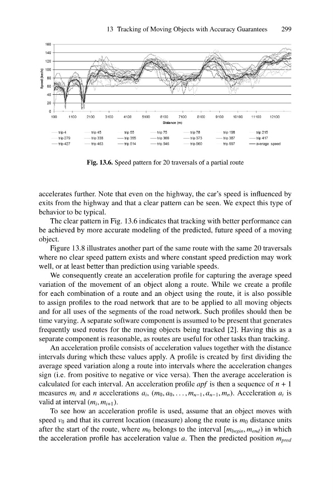
Fig. 13.6. Speed pattern for 20 traversals of a partial route
accelerates further. Note that even on the highway, the car’s speed is influenced by
exits from the highway and that a clear pattern can be seen. We expect this type of
behavior to be typical.
The clear pattern in Fig. 13.6 indicates that tracking with better performance can
be achieved by more accurate modeling of the predicted, future speed of a moving
object.
Figure 13.8 illustrates another part of the same route with the same 20 traversals
where no clear speed pattern exists and where constant speed prediction may work
well, or at least better than prediction using variable speeds.
We consequently create an acceleration profile for capturing the average speed
variation of the movement of an object along a route. While we create a profile
for each combination of a route and an object using the route, it is also possible
to assign profiles to the road network that are to be applied to all moving objects
and for all uses of the segments of the road network. Such profiles should then be
time varying. A separate software component is assumed to be present that generates
frequently used routes for the moving objects being tracked [2]. Having this as a
separate component is reasonable, as routes are useful for other tasks than tracking.
An acceleration profile consists of acceleration values together with the distance
intervals during which these values apply. A profile is created by first dividing the
average speed variation along a route into intervals where the acceleration changes
sign (i.e. from positive to negative or vice versa). Then the average acceleration is
calculated for each interval. An acceleration profile apf is then a sequence of n + 1
measures m i and n accelerations a i , (m 0 , a 0 , . . . , m n−1 , a n−1 , m n ). Acceleration a i is
valid at interval (m i , m i+1 ).
To see how an acceleration profile is used, assume that an object moves with
speed v 0 and that its current location (measure) along the route is m 0 distance units
after the start of the route, where m 0 belongs to the interval [m begin , m end ) in which
the acceleration profile has acceleration value a. Then the predicted position m pred
299
Fig. 13.6. Speed pattern for 20 traversals of a partial route
accelerates further. Note that even on the highway, the car’s speed is influenced by
exits from the highway and that a clear pattern can be seen. We expect this type of
behavior to be typical.
The clear pattern in Fig. 13.6 indicates that tracking with better performance can
be achieved by more accurate modeling of the predicted, future speed of a moving
object.
Figure 13.8 illustrates another part of the same route with the same 20 traversals
where no clear speed pattern exists and where constant speed prediction may work
well, or at least better than prediction using variable speeds.
We consequently create an acceleration profile for capturing the average speed
variation of the movement of an object along a route. While we create a profile
for each combination of a route and an object using the route, it is also possible
to assign profiles to the road network that are to be applied to all moving objects
and for all uses of the segments of the road network. Such profiles should then be
time varying. A separate software component is assumed to be present that generates
frequently used routes for the moving objects being tracked [2]. Having this as a
separate component is reasonable, as routes are useful for other tasks than tracking.
An acceleration profile consists of acceleration values together with the distance
intervals during which these values apply. A profile is created by first dividing the
average speed variation along a route into intervals where the acceleration changes
sign (i.e. from positive to negative or vice versa). Then the average acceleration is
calculated for each interval. An acceleration profile apf is then a sequence of n + 1
measures m i and n accelerations a i , (m 0 , a 0 , . . . , m n−1 , a n−1 , m n ). Acceleration a i is
valid at interval (m i , m i+1 ).
To see how an acceleration profile is used, assume that an object moves with
speed v 0 and that its current location (measure) along the route is m 0 distance units
after the start of the route, where m 0 belongs to the interval [m begin , m end ) in which
the acceleration profile has acceleration value a. Then the predicted position m pred