

298
Alminas ˇ
Civilis, Christian S. Jensen, and Stardas Pakalnis
13.6 Update Reduction Using Acceleration Profiles
Even if the future trajectory of an object is known precisely and updates caused by
segment changes thus are eliminated, updates still occur due to variations in speed.
The reason is that segment-based tracking assumes that objects move at constant
speed – it takes an update to change the speed.
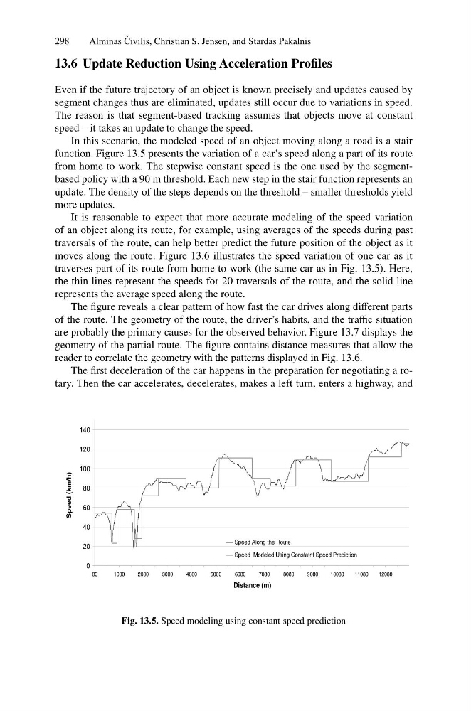
In this scenario, the modeled speed of an object moving along a road is a stair
function. Figure 13.5 presents the variation of a car’s speed along a part of its route
from home to work. The stepwise constant speed is the one used by the segmentbased policy with a 90 m threshold. Each new step in the stair function represents an
update. The density of the steps depends on the threshold – smaller thresholds yield
more updates.
It is reasonable to expect that more accurate modeling of the speed variation
of an object along its route, for example, using averages of the speeds during past
traversals of the route, can help better predict the future position of the object as it
moves along the route. Figure 13.6 illustrates the speed variation of one car as it
traverses part of its route from home to work (the same car as in Fig. 13.5). Here,
the thin lines represent the speeds for 20 traversals of the route, and the solid line
represents the average speed along the route.
The figure reveals a clear pattern of how fast the car drives along different parts
of the route. The geometry of the route, the driver’s habits, and the traffic situation
are probably the primary causes for the observed behavior. Figure 13.7 displays the
geometry of the partial route. The figure contains distance measures that allow the
reader to correlate the geometry with the patterns displayed in Fig. 13.6.
The first deceleration of the car happens in the preparation for negotiating a rotary. Then the car accelerates, decelerates, makes a left turn, enters a highway, and
0
20
40
60
80
100
120
140
80
1080
2080
3080
4080
5080
6080
7080
8080
9080
10080
11080
12080
Distance (m)
Speed (km/h)
Speed Along the Route
Speed Modeled Using Constatnt Speed Prediction
Fig. 13.5. Speed modeling using constant speed prediction
Alminas ˇ
Civilis, Christian S. Jensen, and Stardas Pakalnis
13.6 Update Reduction Using Acceleration Profiles
Even if the future trajectory of an object is known precisely and updates caused by
segment changes thus are eliminated, updates still occur due to variations in speed.
The reason is that segment-based tracking assumes that objects move at constant
speed – it takes an update to change the speed.
In this scenario, the modeled speed of an object moving along a road is a stair
function. Figure 13.5 presents the variation of a car’s speed along a part of its route
from home to work. The stepwise constant speed is the one used by the segmentbased policy with a 90 m threshold. Each new step in the stair function represents an
update. The density of the steps depends on the threshold – smaller thresholds yield
more updates.
It is reasonable to expect that more accurate modeling of the speed variation
of an object along its route, for example, using averages of the speeds during past
traversals of the route, can help better predict the future position of the object as it
moves along the route. Figure 13.6 illustrates the speed variation of one car as it
traverses part of its route from home to work (the same car as in Fig. 13.5). Here,
the thin lines represent the speeds for 20 traversals of the route, and the solid line
represents the average speed along the route.
The figure reveals a clear pattern of how fast the car drives along different parts
of the route. The geometry of the route, the driver’s habits, and the traffic situation
are probably the primary causes for the observed behavior. Figure 13.7 displays the
geometry of the partial route. The figure contains distance measures that allow the
reader to correlate the geometry with the patterns displayed in Fig. 13.6.
The first deceleration of the car happens in the preparation for negotiating a rotary. Then the car accelerates, decelerates, makes a left turn, enters a highway, and
0
20
40
60
80
100
120
140
80
1080
2080
3080
4080
5080
6080
7080
8080
9080
10080
11080
12080
Distance (m)
Speed (km/h)
Speed Along the Route
Speed Modeled Using Constatnt Speed Prediction
Fig. 13.5. Speed modeling using constant speed prediction