

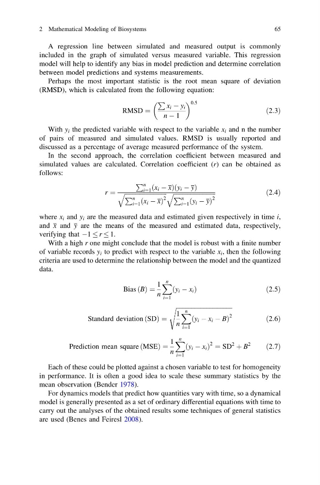
A regression line between simulated and measured output is commonly
included in the graph of simulated versus measured variable. This regression
model will help to identify any bias in model prediction and determine correlation
between model predictions and systems measurements.
Perhaps the most important statistic is the root mean square of deviation
(RMSD), which is calculated from the following equation:
RMSD ¼
P
x i À y i
n À 1
0:5
ð2:3Þ
With y i the predicted variable with respect to the variable x i and n the number
of pairs of measured and simulated values. RMSD is usually reported and
discussed as a percentage of average measured performance of the system.
In the second approach, the correlation coefficient between measured and
simulated values are calculated. Correlation coefficient (r) can be obtained as
follows:
r ¼
P n
i¼1 x i À x
ð
Þ y i À y
ð
Þ
ffiffiffiffiffiffiffiffiffiffiffiffiffiffiffiffiffiffiffiffiffiffiffiffiffiffiffi ffi
P n
i¼1 x i À x
ð
Þ
2
q
ffiffiffiffiffiffiffiffiffiffiffiffiffiffiffiffiffiffiffiffiffiffiffiffiffiffiffi ffi
P n
i¼1 y i À y
ð
Þ
2
q
ð2:4Þ
where x i and y i are the measured data and estimated given respectively in time i,
and x and y are the means of the measured and estimated data, respectively,
verifying that À1 r 1.
With a high r one might conclude that the model is robust with a finite number
of variable records y i to predict with respect to the variable x i , then the following
criteria are used to determine the relationship between the model and the quantized
data.
Bias B
ð Þ ¼
1
n
X n
i¼1
ðy i À x i Þ
ð 2:5Þ
Standard deviation SD
ð Þ ¼
ffiffiffiffiffiffiffiffiffiffiffiffiffiffiffiffiffiffiffiffiffiffiffiffiffiffiffiffiffiffiffiffiffiffiffiffiffi
1
n
X n
i¼1
ðy i À x i À BÞ
2
s
ð2:6Þ
Prediction mean square MSE
ð
Þ¼
1
n
X n
i¼1
ðy i À x i Þ
2 ¼ SD
2 þ B
2
ð2:7Þ
Each of these could be plotted against a chosen variable to test for homogeneity
in performance. It is often a good idea to scale these summary statistics by the
mean observation (Bender 1978).
For dynamics models that predict how quantities vary with time, so a dynamical
model is generally presented as a set of ordinary differential equations with time to
carry out the analyses of the obtained results some techniques of general statistics
are used (Benes and Feiresl 2008).
2 Mathematical Modeling of Biosystems
65
included in the graph of simulated versus measured variable. This regression
model will help to identify any bias in model prediction and determine correlation
between model predictions and systems measurements.
Perhaps the most important statistic is the root mean square of deviation
(RMSD), which is calculated from the following equation:
RMSD ¼
P
x i À y i
n À 1
0:5
ð2:3Þ
With y i the predicted variable with respect to the variable x i and n the number
of pairs of measured and simulated values. RMSD is usually reported and
discussed as a percentage of average measured performance of the system.
In the second approach, the correlation coefficient between measured and
simulated values are calculated. Correlation coefficient (r) can be obtained as
follows:
r ¼
P n
i¼1 x i À x
ð
Þ y i À y
ð
Þ
ffiffiffiffiffiffiffiffiffiffiffiffiffiffiffiffiffiffiffiffiffiffiffiffiffiffiffi ffi
P n
i¼1 x i À x
ð
Þ
2
q
ffiffiffiffiffiffiffiffiffiffiffiffiffiffiffiffiffiffiffiffiffiffiffiffiffiffiffi ffi
P n
i¼1 y i À y
ð
Þ
2
q
ð2:4Þ
where x i and y i are the measured data and estimated given respectively in time i,
and x and y are the means of the measured and estimated data, respectively,
verifying that À1 r 1.
With a high r one might conclude that the model is robust with a finite number
of variable records y i to predict with respect to the variable x i , then the following
criteria are used to determine the relationship between the model and the quantized
data.
Bias B
ð Þ ¼
1
n
X n
i¼1
ðy i À x i Þ
ð 2:5Þ
Standard deviation SD
ð Þ ¼
ffiffiffiffiffiffiffiffiffiffiffiffiffiffiffiffiffiffiffiffiffiffiffiffiffiffiffiffiffiffiffiffiffiffiffiffiffi
1
n
X n
i¼1
ðy i À x i À BÞ
2
s
ð2:6Þ
Prediction mean square MSE
ð
Þ¼
1
n
X n
i¼1
ðy i À x i Þ
2 ¼ SD
2 þ B
2
ð2:7Þ
Each of these could be plotted against a chosen variable to test for homogeneity
in performance. It is often a good idea to scale these summary statistics by the
mean observation (Bender 1978).
For dynamics models that predict how quantities vary with time, so a dynamical
model is generally presented as a set of ordinary differential equations with time to
carry out the analyses of the obtained results some techniques of general statistics
are used (Benes and Feiresl 2008).
2 Mathematical Modeling of Biosystems
65