

timescales (van Henten and Bontsema 2009), it is necessary to state and solve an
optimal control problem with slow dynamics to solve the long-term seasonal
optimization taking into consideration the crop model and also a problem with fast
dynamics to solve the short-term optimization problem using the greenhouse climate model. Researchers such as Seginer and Ioslovich (1998); Chalabi et al.
(1996); Ioslovich and Seginer (1996) calculated suboptimal solutions given that
their studies were focused only on the long-term optimization. On the other hand,
van Henten (1994) proposed, the first time, the use of singularly perturbation
systems theory stating and solving the open-loop optimal control problem in
greenhouses. Tap (2000) proposed two timescales decomposition for the greenhouse optimal control problem. Also, Van Willigenburg et al. (2000) used three
timescales. The numerical methods used to solve the dynamic optimization
problem of the greenhouse climate have been mainly gradient-based methods
(Bryson 1999). The solution of the optimal control problem of greenhouse climate
using two timescales proceeds as follows (van Henten and Bontsema 1996, 2009):
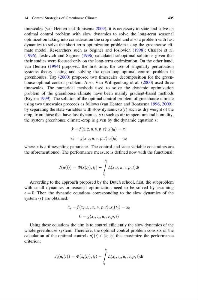
by separating the state variables with slow dynamics xðtÞ such as dry weight of the
crop, from those that have fast dynamics zðtÞ such as air temperature and humidity,
the system greenhouse climate-crop is given by the dynamic equation s:
_
x ¼ f ðx; z; u; v; p; tÞ; xðt 0 Þ ¼ x 0
e_ z ¼ gðx; z; u; v; p; tÞ; zðt 0 Þ ¼ z 0
where e is a timescaling parameter. The control and state variable constraints are
the aforementioned. The performance measure is defined now with the functional:
JðuðtÞÞ ¼ Uðxðt f Þ; t f Þ þ
Z t f
t 0
Lðx; z; u; v; p; tÞdt
According to the approach proposed by the Dutch school, first, the subproblem
with small dynamics or seasonal optimization need to be solved by assuming
e ¼ 0. Then the dynamic equations corresponding to the slow dynamics of the
system (s) are obtained:
_
x s ¼ f ðx s ; z s ; u s ; v; p; tÞ; x s ðt 0 Þ ¼ x 0
0 ¼ gðx s ; z s ; u s ; v; p; tÞ
Using these equations the aim is to control efficiently the slow dynamics of the
whole greenhouse system. Therefore, the optimal control problem consists of the
calculation of the optimal controls u
Ã
s ðtÞ 2 ½t 0 ; t f that maximize the performance
criterion:
J s ðu s ðtÞÞ ¼ Uðx s ðt f Þ; t f Þ À
Z t f
t 0
Lðx s ; z s ; u s ; v; p; tÞdt
14 Control Strategies of Greenhouse Climate
405
optimal control problem with slow dynamics to solve the long-term seasonal
optimization taking into consideration the crop model and also a problem with fast
dynamics to solve the short-term optimization problem using the greenhouse climate model. Researchers such as Seginer and Ioslovich (1998); Chalabi et al.
(1996); Ioslovich and Seginer (1996) calculated suboptimal solutions given that
their studies were focused only on the long-term optimization. On the other hand,
van Henten (1994) proposed, the first time, the use of singularly perturbation
systems theory stating and solving the open-loop optimal control problem in
greenhouses. Tap (2000) proposed two timescales decomposition for the greenhouse optimal control problem. Also, Van Willigenburg et al. (2000) used three
timescales. The numerical methods used to solve the dynamic optimization
problem of the greenhouse climate have been mainly gradient-based methods
(Bryson 1999). The solution of the optimal control problem of greenhouse climate
using two timescales proceeds as follows (van Henten and Bontsema 1996, 2009):
by separating the state variables with slow dynamics xðtÞ such as dry weight of the
crop, from those that have fast dynamics zðtÞ such as air temperature and humidity,
the system greenhouse climate-crop is given by the dynamic equation s:
_
x ¼ f ðx; z; u; v; p; tÞ; xðt 0 Þ ¼ x 0
e_ z ¼ gðx; z; u; v; p; tÞ; zðt 0 Þ ¼ z 0
where e is a timescaling parameter. The control and state variable constraints are
the aforementioned. The performance measure is defined now with the functional:
JðuðtÞÞ ¼ Uðxðt f Þ; t f Þ þ
Z t f
t 0
Lðx; z; u; v; p; tÞdt
According to the approach proposed by the Dutch school, first, the subproblem
with small dynamics or seasonal optimization need to be solved by assuming
e ¼ 0. Then the dynamic equations corresponding to the slow dynamics of the
system (s) are obtained:
_
x s ¼ f ðx s ; z s ; u s ; v; p; tÞ; x s ðt 0 Þ ¼ x 0
0 ¼ gðx s ; z s ; u s ; v; p; tÞ
Using these equations the aim is to control efficiently the slow dynamics of the
whole greenhouse system. Therefore, the optimal control problem consists of the
calculation of the optimal controls u
Ã
s ðtÞ 2 ½t 0 ; t f that maximize the performance
criterion:
J s ðu s ðtÞÞ ¼ Uðx s ðt f Þ; t f Þ À
Z t f
t 0
Lðx s ; z s ; u s ; v; p; tÞdt
14 Control Strategies of Greenhouse Climate
405