

14.2.2 Solution Methods
The solution methods applied to the optimal control of a greenhouse system are
numerical and they are classified in indirect methods (Bryson 1999) which use the
Pontryagin minimum principle (Seginer et al. 1991; Seginer and McClendon 1992;
Seginer 1996; van Henten 1994; van Henten et al. 1997a, b; Trigui et al. 2001a, b;
Ioslovich and Seginer 2002; Ioslovich et al. 2009) and direct methods (Bryson
1999) which transform the original optimal control problem in a nonlinear programming (NLP) problem (Chalabi et al. 1996, 2002a, b). According to the literature the first approach has been applied mostly to the greenhouse system.
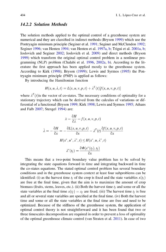
According to Kirk (1998); Bryson (1999); Lewis and Syrmos (1995) the Pontryagin minimum principle (PMP) is applied as follows:
By introducing the Hamiltonian function
Hðx; u; k; tÞ ¼ Lðx; u; v; p; tÞ þ k
T ðtÞ f ðx; u; v; p; tÞ
½
where k
T ðtÞis the vector of co-states. The necessary conditions of optimality for a
stationary trajectory which can be derived from the calculus of variations or differential of a functional (Bryson 1999; Kirk 1998; Lewis and Syrmos 1995; Athans
and Falb 2007; Stengel 1994) are:
_
x ¼
oH
ok
¼ f ðx; u; v; p; tÞ
_
k ¼ À
oH
ox
¼ À
oLðx; u; v; p; tÞ
ox
À k
T ðtÞ
of ðx; u; v; p; tÞ
ox
Hðx
à ; u
à ; k
à ; tÞ Hðx
à ; u; k
à ; tÞ
k
à ðt f Þ ¼
oUðx
à ðt f Þ; t f Þ
ox
This means that a two-point boundary value problem has to be solved by
integrating the state equations forward in time and integrating backward in time
the co-states equations. The stated optimal control problem has several boundary
conditions and in the greenhouse system context at least four subproblems can be
identified: (i) as the harvest time t f of the crop is fixed and the state variables xðt f Þ
are free at the final time, given that the aim is to maximize the amount of crop
biomass (fruits, stems, leaves, etc.). (ii) Both the harvest time t f and some or all the
state variables at the final time xðt f Þ ¼ x f are fixed. (iii) The harvest time t f is free
and all or several state variables are specified at the final time. (iv) Both the harvest
time and some or all the state variables at the final time are free and need to be
optimized. Because of the stiffness of the greenhouse system, the application of
optimal control theory is not straightforward and it has been found that two or
three timescales decomposition are required in order to prevent a loss of optimality
of the optimal greenhouse climate control (van Straten et al. 2011). In case of two
404
I. L. López-Cruz et al.
The solution methods applied to the optimal control of a greenhouse system are
numerical and they are classified in indirect methods (Bryson 1999) which use the
Pontryagin minimum principle (Seginer et al. 1991; Seginer and McClendon 1992;
Seginer 1996; van Henten 1994; van Henten et al. 1997a, b; Trigui et al. 2001a, b;
Ioslovich and Seginer 2002; Ioslovich et al. 2009) and direct methods (Bryson
1999) which transform the original optimal control problem in a nonlinear programming (NLP) problem (Chalabi et al. 1996, 2002a, b). According to the literature the first approach has been applied mostly to the greenhouse system.
According to Kirk (1998); Bryson (1999); Lewis and Syrmos (1995) the Pontryagin minimum principle (PMP) is applied as follows:
By introducing the Hamiltonian function
Hðx; u; k; tÞ ¼ Lðx; u; v; p; tÞ þ k
T ðtÞ f ðx; u; v; p; tÞ
½
where k
T ðtÞis the vector of co-states. The necessary conditions of optimality for a
stationary trajectory which can be derived from the calculus of variations or differential of a functional (Bryson 1999; Kirk 1998; Lewis and Syrmos 1995; Athans
and Falb 2007; Stengel 1994) are:
_
x ¼
oH
ok
¼ f ðx; u; v; p; tÞ
_
k ¼ À
oH
ox
¼ À
oLðx; u; v; p; tÞ
ox
À k
T ðtÞ
of ðx; u; v; p; tÞ
ox
Hðx
à ; u
à ; k
à ; tÞ Hðx
à ; u; k
à ; tÞ
k
à ðt f Þ ¼
oUðx
à ðt f Þ; t f Þ
ox
This means that a two-point boundary value problem has to be solved by
integrating the state equations forward in time and integrating backward in time
the co-states equations. The stated optimal control problem has several boundary
conditions and in the greenhouse system context at least four subproblems can be
identified: (i) as the harvest time t f of the crop is fixed and the state variables xðt f Þ
are free at the final time, given that the aim is to maximize the amount of crop
biomass (fruits, stems, leaves, etc.). (ii) Both the harvest time t f and some or all the
state variables at the final time xðt f Þ ¼ x f are fixed. (iii) The harvest time t f is free
and all or several state variables are specified at the final time. (iv) Both the harvest
time and some or all the state variables at the final time are free and need to be
optimized. Because of the stiffness of the greenhouse system, the application of
optimal control theory is not straightforward and it has been found that two or
three timescales decomposition are required in order to prevent a loss of optimality
of the optimal greenhouse climate control (van Straten et al. 2011). In case of two
404
I. L. López-Cruz et al.