

system (H), fogging system, ventilation system, cooling system, or CO 2 injection
(/ i ). Formalizing the main ideas aforementioned (van Henten 1994; Tap 2000) a
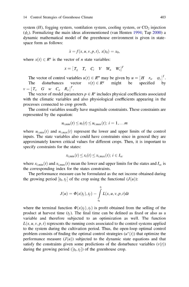
dynamic mathematical model of the greenhouse environment is given in statespace form as follows:
_
x ¼ f ðx; u; v; p; tÞ; xðt 0 Þ ¼ x 0 ;
where xðtÞ 2 R
n is the vector of n state variables:
x ¼ ½ T g T s C i V W n W s
T
The vector of control variables uðtÞ 2 R
m may be given by u ¼ ½ H r w u i
T .
The
disturbances
vector
vðtÞ 2 R
q
might
be
specified
by
v ¼ ½ T o G w C o R o
T .
The vector of model parameters p 2 R
s includes physical coefficients associated
with the climatic variables and also physiological coefficients appearing in the
processes connected to crop growth.
The control variables usually have magnitude constraints. These constraints are
represented by the equation:
u i;min ðtÞ u i ðtÞ u i;max ðtÞ; i ¼ 1; . . .m
where u i;min ðtÞ and u i;max ðtÞ represent the lower and upper limits of the control
inputs. The state variables also could have constraints since in general they are
approximately known critical values for different crops. Then, it is important to
specify constraints for the states:
x i;min ðtÞ x i ðtÞ x i;max ðtÞ; i 2 I xc
where x i;min ðtÞ and x i;max ðtÞ mean the lower and upper limits for the states and I xc is
the corresponding index for the states constraints.
The performance measure can be formulated as the net income obtained during
the growing period ½t 0 ; t f of the crop using the functional (JðuÞ):
JðuÞ ¼ Uðxðt f Þ; t f Þ À
Z t f
t 0
Lðx; u; v; p; tÞdt
where the terminal function Uðxðt f Þ; t f Þ is profit obtained from the selling of the
product at harvest time (t f ). The final time can be defined as fixed or also as a
variable and therefore subjected to an optimization as well. The function
Lðx; u; v; p; tÞ represents the running costs associated to the control systems applied
to the system during the cultivation period. Thus, the open-loop optimal control
problem consists of finding the optimal control strategies (u
à ðtÞ) that optimize the
performance measure (JðuÞ) subjected to the dynamic state equations and that
satisfy the constraints given some predictions of the disturbance variables (vðtÞ)
during the growing period (½t 0 ; t f ) of the greenhouse crop.
14 Control Strategies of Greenhouse Climate
403
(/ i ). Formalizing the main ideas aforementioned (van Henten 1994; Tap 2000) a
dynamic mathematical model of the greenhouse environment is given in statespace form as follows:
_
x ¼ f ðx; u; v; p; tÞ; xðt 0 Þ ¼ x 0 ;
where xðtÞ 2 R
n is the vector of n state variables:
x ¼ ½ T g T s C i V W n W s
T
The vector of control variables uðtÞ 2 R
m may be given by u ¼ ½ H r w u i
T .
The
disturbances
vector
vðtÞ 2 R
q
might
be
specified
by
v ¼ ½ T o G w C o R o
T .
The vector of model parameters p 2 R
s includes physical coefficients associated
with the climatic variables and also physiological coefficients appearing in the
processes connected to crop growth.
The control variables usually have magnitude constraints. These constraints are
represented by the equation:
u i;min ðtÞ u i ðtÞ u i;max ðtÞ; i ¼ 1; . . .m
where u i;min ðtÞ and u i;max ðtÞ represent the lower and upper limits of the control
inputs. The state variables also could have constraints since in general they are
approximately known critical values for different crops. Then, it is important to
specify constraints for the states:
x i;min ðtÞ x i ðtÞ x i;max ðtÞ; i 2 I xc
where x i;min ðtÞ and x i;max ðtÞ mean the lower and upper limits for the states and I xc is
the corresponding index for the states constraints.
The performance measure can be formulated as the net income obtained during
the growing period ½t 0 ; t f of the crop using the functional (JðuÞ):
JðuÞ ¼ Uðxðt f Þ; t f Þ À
Z t f
t 0
Lðx; u; v; p; tÞdt
where the terminal function Uðxðt f Þ; t f Þ is profit obtained from the selling of the
product at harvest time (t f ). The final time can be defined as fixed or also as a
variable and therefore subjected to an optimization as well. The function
Lðx; u; v; p; tÞ represents the running costs associated to the control systems applied
to the system during the cultivation period. Thus, the open-loop optimal control
problem consists of finding the optimal control strategies (u
à ðtÞ) that optimize the
performance measure (JðuÞ) subjected to the dynamic state equations and that
satisfy the constraints given some predictions of the disturbance variables (vðtÞ)
during the growing period (½t 0 ; t f ) of the greenhouse crop.
14 Control Strategies of Greenhouse Climate
403