

subjected to the slow dynamics equations and states and controls constraints.
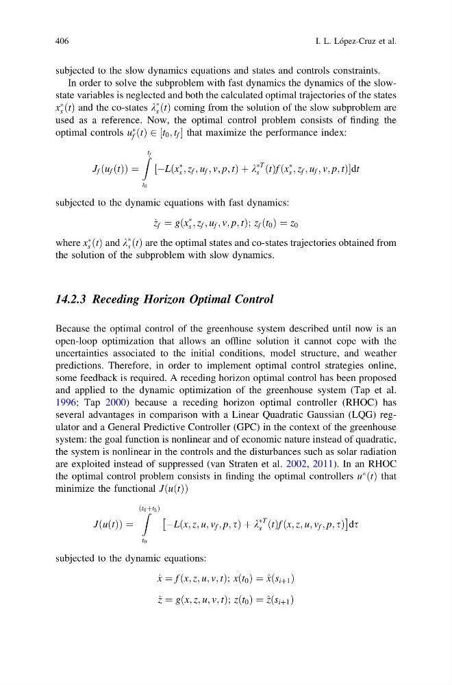
In order to solve the subproblem with fast dynamics the dynamics of the slowstate variables is neglected and both the calculated optimal trajectories of the states
x
Ã
s ðtÞ and the co-states k
Ã
s ðtÞ coming from the solution of the slow subproblem are
used as a reference. Now, the optimal control problem consists of finding the
optimal controls u
Ã
f ðtÞ 2 ½t 0 ; t f that maximize the performance index:
J f ðu f ðtÞÞ ¼
Z t f
t 0
½ÀLðx
Ã
s ; z f ; u f ; v; p; tÞ þ k
ÃT
s ðtÞf ðx
Ã
s ; z f ; u f ; v; p; tÞdt
subjected to the dynamic equations with fast dynamics:
_
z f ¼ gðx
Ã
s ; z f ; u f ; v; p; tÞ; z f ðt 0 Þ ¼ z 0
where x
Ã
s ðtÞ and k
Ã
s ðtÞ are the optimal states and co-states trajectories obtained from
the solution of the subproblem with slow dynamics.
14.2.3 Receding Horizon Optimal Control
Because the optimal control of the greenhouse system described until now is an
open-loop optimization that allows an offline solution it cannot cope with the
uncertainties associated to the initial conditions, model structure, and weather
predictions. Therefore, in order to implement optimal control strategies online,
some feedback is required. A receding horizon optimal control has been proposed
and applied to the dynamic optimization of the greenhouse system (Tap et al.
1996; Tap 2000) because a receding horizon optimal controller (RHOC) has
several advantages in comparison with a Linear Quadratic Gaussian (LQG) regulator and a General Predictive Controller (GPC) in the context of the greenhouse
system: the goal function is nonlinear and of economic nature instead of quadratic,
the system is nonlinear in the controls and the disturbances such as solar radiation
are exploited instead of suppressed (van Straten et al. 2002, 2011). In an RHOC
the optimal control problem consists in finding the optimal controllers u
à ðtÞ that
minimize the functional JðuðtÞÞ
JðuðtÞÞ ¼
Z
ðt 0 þt h Þ
t 0
ÀLðx; z; u; v f ; p; sÞ þ k
ÃT
s ðtÞf ðx; z; u; v f ; p; sÞ
Â
Ã
ds
subjected to the dynamic equations:
_
x ¼ f ðx; z; u; v; tÞ; xðt 0 Þ ¼ ^ xðs iþ1 Þ
_
z ¼ gðx; z; u; v; tÞ; zðt 0 Þ ¼ ^ zðs iþ1 Þ
406
I. L. López-Cruz et al.
In order to solve the subproblem with fast dynamics the dynamics of the slowstate variables is neglected and both the calculated optimal trajectories of the states
x
Ã
s ðtÞ and the co-states k
Ã
s ðtÞ coming from the solution of the slow subproblem are
used as a reference. Now, the optimal control problem consists of finding the
optimal controls u
Ã
f ðtÞ 2 ½t 0 ; t f that maximize the performance index:
J f ðu f ðtÞÞ ¼
Z t f
t 0
½ÀLðx
Ã
s ; z f ; u f ; v; p; tÞ þ k
ÃT
s ðtÞf ðx
Ã
s ; z f ; u f ; v; p; tÞdt
subjected to the dynamic equations with fast dynamics:
_
z f ¼ gðx
Ã
s ; z f ; u f ; v; p; tÞ; z f ðt 0 Þ ¼ z 0
where x
Ã
s ðtÞ and k
Ã
s ðtÞ are the optimal states and co-states trajectories obtained from
the solution of the subproblem with slow dynamics.
14.2.3 Receding Horizon Optimal Control
Because the optimal control of the greenhouse system described until now is an
open-loop optimization that allows an offline solution it cannot cope with the
uncertainties associated to the initial conditions, model structure, and weather
predictions. Therefore, in order to implement optimal control strategies online,
some feedback is required. A receding horizon optimal control has been proposed
and applied to the dynamic optimization of the greenhouse system (Tap et al.
1996; Tap 2000) because a receding horizon optimal controller (RHOC) has
several advantages in comparison with a Linear Quadratic Gaussian (LQG) regulator and a General Predictive Controller (GPC) in the context of the greenhouse
system: the goal function is nonlinear and of economic nature instead of quadratic,
the system is nonlinear in the controls and the disturbances such as solar radiation
are exploited instead of suppressed (van Straten et al. 2002, 2011). In an RHOC
the optimal control problem consists in finding the optimal controllers u
à ðtÞ that
minimize the functional JðuðtÞÞ
JðuðtÞÞ ¼
Z
ðt 0 þt h Þ
t 0
ÀLðx; z; u; v f ; p; sÞ þ k
ÃT
s ðtÞf ðx; z; u; v f ; p; sÞ
Â
Ã
ds
subjected to the dynamic equations:
_
x ¼ f ðx; z; u; v; tÞ; xðt 0 Þ ¼ ^ xðs iþ1 Þ
_
z ¼ gðx; z; u; v; tÞ; zðt 0 Þ ¼ ^ zðs iþ1 Þ
406
I. L. López-Cruz et al.