

270
J. M. Magalhaes et al.
Baines (1982) barotropic tidal forcing is often used to search and identify hotspot
regions of ISWs within a given study area. It has proved to be a valuable indicator
in several other independent studies, particularly to study the possibility of the local
generation mechanism. For instance, Azevedo et al. (2006) and da Silva et al. (2007)
have used this method to investigate the local generation mechanism in the southern
Bay of Biscay (near Cape Finisterre), and in the southern slopes of the Estremadura
Promontory (off the west Iberian shelf). In addition, there have been other authors that
also used this technique over the last decade, as a valuable indicator of where large
ITs may be generated (e.g. Colosi et al. 2001; Merrifield and Holloway 2002; Niwa
and Hibiya 2004). On the other hand, ray-tracing techniques are used to see if the
locations where ISWs first appear are consistent with the local generation mechanism
(i.e. if the first ISW packets appear a few kilometers ahead of the expected impact
of an IT beam with the pycnocline). Note that, ITs in a continuously stratified ocean
can be described by beams or rays that follow characteristic pathways (along which
their energy can propagate—see Eq. 14.1). In other words, this means that when the
bottom slopes match the local value of tan(θ) (called a critical region) the generation
of ITs is more pronounced, particularly if the barotropic currents are strong. In
such cases, the direction of the forcing barotropic flow is then coincident with the
motion plane for free internal waves, resulting in resonant conditions and enhanced
generation of the ITs and ISWs.
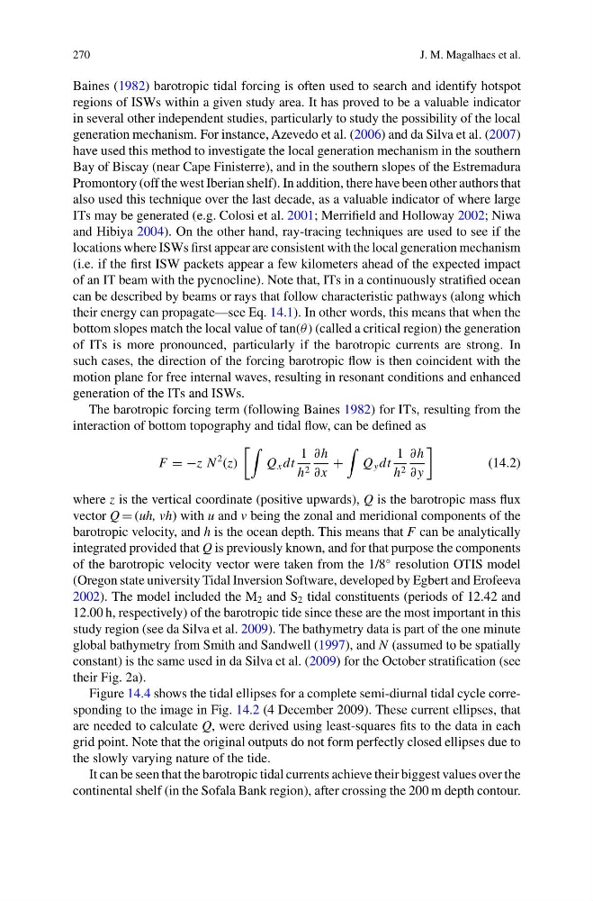
The barotropic forcing term (following Baines 1982) for ITs, resulting from the
interaction of bottom topography and tidal flow, can be defined as
F = −z N
2 (z)
Q x dt
1
h 2
∂h
∂x
+
Q y dt
1
h 2
∂h
∂y
(14.2)
where z is the vertical coordinate (positive upwards), Q is the barotropic mass flux
vector Q = (uh, vh) with u and v being the zonal and meridional components of the
barotropic velocity, and h is the ocean depth. This means that F can be analytically
integrated provided that Q is previously known, and for that purpose the components
of the barotropic velocity vector were taken from the 1/8
◦ resolution OTIS model
(Oregon state university Tidal Inversion Software, developed by Egbert and Erofeeva
2002). The model included the M 2 and S 2 tidal constituents (periods of 12.42 and
12.00 h, respectively) of the barotropic tide since these are the most important in this
study region (see da Silva et al. 2009). The bathymetry data is part of the one minute
global bathymetry from Smith and Sandwell (1997), and N (assumed to be spatially
constant) is the same used in da Silva et al. (2009) for the October stratification (see
their Fig. 2a).
Figure 14.4 shows the tidal ellipses for a complete semi-diurnal tidal cycle corresponding to the image in Fig. 14.2 (4 December 2009). These current ellipses, that
are needed to calculate Q, were derived using least-squares fits to the data in each
grid point. Note that the original outputs do not form perfectly closed ellipses due to
the slowly varying nature of the tide.
It can be seen that the barotropic tidal currents achieve their biggest values over the
continental shelf (in the Sofala Bank region), after crossing the 200 m depth contour.
J. M. Magalhaes et al.
Baines (1982) barotropic tidal forcing is often used to search and identify hotspot
regions of ISWs within a given study area. It has proved to be a valuable indicator
in several other independent studies, particularly to study the possibility of the local
generation mechanism. For instance, Azevedo et al. (2006) and da Silva et al. (2007)
have used this method to investigate the local generation mechanism in the southern
Bay of Biscay (near Cape Finisterre), and in the southern slopes of the Estremadura
Promontory (off the west Iberian shelf). In addition, there have been other authors that
also used this technique over the last decade, as a valuable indicator of where large
ITs may be generated (e.g. Colosi et al. 2001; Merrifield and Holloway 2002; Niwa
and Hibiya 2004). On the other hand, ray-tracing techniques are used to see if the
locations where ISWs first appear are consistent with the local generation mechanism
(i.e. if the first ISW packets appear a few kilometers ahead of the expected impact
of an IT beam with the pycnocline). Note that, ITs in a continuously stratified ocean
can be described by beams or rays that follow characteristic pathways (along which
their energy can propagate—see Eq. 14.1). In other words, this means that when the
bottom slopes match the local value of tan(θ) (called a critical region) the generation
of ITs is more pronounced, particularly if the barotropic currents are strong. In
such cases, the direction of the forcing barotropic flow is then coincident with the
motion plane for free internal waves, resulting in resonant conditions and enhanced
generation of the ITs and ISWs.
The barotropic forcing term (following Baines 1982) for ITs, resulting from the
interaction of bottom topography and tidal flow, can be defined as
F = −z N
2 (z)
Q x dt
1
h 2
∂h
∂x
+
Q y dt
1
h 2
∂h
∂y
(14.2)
where z is the vertical coordinate (positive upwards), Q is the barotropic mass flux
vector Q = (uh, vh) with u and v being the zonal and meridional components of the
barotropic velocity, and h is the ocean depth. This means that F can be analytically
integrated provided that Q is previously known, and for that purpose the components
of the barotropic velocity vector were taken from the 1/8
◦ resolution OTIS model
(Oregon state university Tidal Inversion Software, developed by Egbert and Erofeeva
2002). The model included the M 2 and S 2 tidal constituents (periods of 12.42 and
12.00 h, respectively) of the barotropic tide since these are the most important in this
study region (see da Silva et al. 2009). The bathymetry data is part of the one minute
global bathymetry from Smith and Sandwell (1997), and N (assumed to be spatially
constant) is the same used in da Silva et al. (2009) for the October stratification (see
their Fig. 2a).
Figure 14.4 shows the tidal ellipses for a complete semi-diurnal tidal cycle corresponding to the image in Fig. 14.2 (4 December 2009). These current ellipses, that
are needed to calculate Q, were derived using least-squares fits to the data in each
grid point. Note that the original outputs do not form perfectly closed ellipses due to
the slowly varying nature of the tide.
It can be seen that the barotropic tidal currents achieve their biggest values over the
continental shelf (in the Sofala Bank region), after crossing the 200 m depth contour.