

3.1. Humpback Whales and Sand Lance
45
components that are in the model do not correspond with each other. For
example, if the change in the whale population were measured in tons of
whale biomass per year and the whale population itself were measured in
number of individuals , then a correspondence between the number of
whales and their bioma ss needs to be established. For example, one could
introduce a new parameter that reflects the average biomass per whale.
Equations (1) and (2) make a number of simplifying assumptions. For instance, the growth of the prey is limited only by predation, predators consume only one species of prey, consumption of prey is unlimited, and
predator and prey encounter one another randomly in a homogeneous environment (Gotelli 1995). Such assumptions are clearly an oversimplification of the conditions under which organisms exist in the natural world .
However, this does not preclude our use of the Lotka-Volterra model for
exploring one way in which two specie s can be thought to interact with
each another.
The Lotka-Volterra equations (1) and (2) provide a convenient starting
point for a model of the inclusion of predator-prey dynamics in our humpback whale population model of Chapter 2. However, before we proceed
to use these equations, we will modify one of them to alleviate one of the
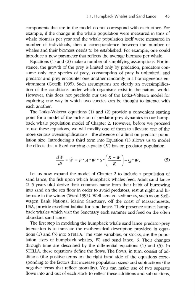
more serious oversimplifications-the absence of a limit on predator population size. Introducing a third term into Equation (1) allows us to model
the effects that a fixed carrying capacity (K) has on predator population.
dW
-:it = W . = F • A • W • S· (K-W) -K-- - Q• W .
(5)
Let us now expand the model of Chapter 2 to include a population of
sand lance, the fish upon which humpback whales feed . Adult sand lance
(2-5 years old) derive their common name from their habit of burrowing
into sand on the sea floor in order to avoid predators, rest at night and hibernate in the winter (Ward 1995). Well-aerated sediments, such as on Stellwagen Bank National Marine Sanctu ary, off the coast of Massachusetts,
USA, provide excellent habitat for sand lance. Their presence attract humpback whales which visit the Sanctuary each summer and feed on the often
abundant sand lance .
The first step in modeling the humpback whale sand lance predator-prey
interaction is to translate the mathematical description provided in equations (1) and (5) into STELLA. The state variables, or stocks, are the population sizes of humpback whales , W; and sand lance , S. Their changes
through time are described by the differential equations (1) and (5). In
STELLA, these equations define the flows. The flows, in turn , consist of additions (the positive terms on the right hand side of the equations corresponding to the factors that increase population sizes) and subtractions (the
negative terms that reflect mortality). You can make use of two separate
flows into and out of each stock to reflect these add itions and subtractions,
45
components that are in the model do not correspond with each other. For
example, if the change in the whale population were measured in tons of
whale biomass per year and the whale population itself were measured in
number of individuals , then a correspondence between the number of
whales and their bioma ss needs to be established. For example, one could
introduce a new parameter that reflects the average biomass per whale.
Equations (1) and (2) make a number of simplifying assumptions. For instance, the growth of the prey is limited only by predation, predators consume only one species of prey, consumption of prey is unlimited, and
predator and prey encounter one another randomly in a homogeneous environment (Gotelli 1995). Such assumptions are clearly an oversimplification of the conditions under which organisms exist in the natural world .
However, this does not preclude our use of the Lotka-Volterra model for
exploring one way in which two specie s can be thought to interact with
each another.
The Lotka-Volterra equations (1) and (2) provide a convenient starting
point for a model of the inclusion of predator-prey dynamics in our humpback whale population model of Chapter 2. However, before we proceed
to use these equations, we will modify one of them to alleviate one of the
more serious oversimplifications-the absence of a limit on predator population size. Introducing a third term into Equation (1) allows us to model
the effects that a fixed carrying capacity (K) has on predator population.
dW
-:it = W . = F • A • W • S· (K-W) -K-- - Q• W .
(5)
Let us now expand the model of Chapter 2 to include a population of
sand lance, the fish upon which humpback whales feed . Adult sand lance
(2-5 years old) derive their common name from their habit of burrowing
into sand on the sea floor in order to avoid predators, rest at night and hibernate in the winter (Ward 1995). Well-aerated sediments, such as on Stellwagen Bank National Marine Sanctu ary, off the coast of Massachusetts,
USA, provide excellent habitat for sand lance. Their presence attract humpback whales which visit the Sanctuary each summer and feed on the often
abundant sand lance .
The first step in modeling the humpback whale sand lance predator-prey
interaction is to translate the mathematical description provided in equations (1) and (5) into STELLA. The state variables, or stocks, are the population sizes of humpback whales , W; and sand lance , S. Their changes
through time are described by the differential equations (1) and (5). In
STELLA, these equations define the flows. The flows, in turn , consist of additions (the positive terms on the right hand side of the equations corresponding to the factors that increase population sizes) and subtractions (the
negative terms that reflect mortality). You can make use of two separate
flows into and out of each stock to reflect these add itions and subtractions,