

2 harvesting
4: Wold Shrimp Biomass
1:
4:
1:
5.00
2
3
J
1 7·5Oe+008 of- -
4: 7.50e+009
- - ' I... - - t - - - -I
1:
4:
402
18 . The Global Shrimp Market
p,
10.00
1.5Oe+OO9
1.5Oe+Ol0
0.00
0.00
----~~----~~----+---0.00
150.00
450 .00
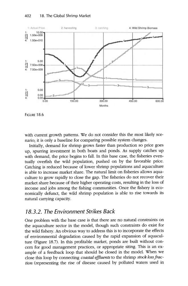
FIGURE 18.6
600.00
with current growth patterns. We do not consider this the most likely scenario; it is only a baseline for comparing possible system changes.
Initially, demand for shrimp grows faster than production so price goes
up , spurring investment in both boats and ponds. As supply catches up
with demand, the price begins to fall. In this base case, the fisheries eventually overfish the wild population, pushed on by the favorable price.
Catching is reduced because of lower shrimp populations and aquaculture
is able to increase market share . The natural limit on fisheries allows aquaculture to grow rapidly to close the gap . The fisheries do not recover their
market share because of their higher operating costs, resulting in the loss of
income and jobs among the fishing communities. Once the fishery is economically defunct , the wild shrimp population is able to rise towards its
natural carrying capacity .
18.3.2. The En vironment Strikes Back
One problem with the base case is that there are no natural constraints on
the aquaculture sector in the model, though such constraints do exist for
the wild fishery. An obvious way to address this is to incorporate the effects
of environmental degradation caused by the rapid expansion of aquaculture (Figure 18.7). In this profitable market, ponds are built without concern for good management practices, or appropriate siting. This is an example of a feedback loop that should be closed in the model. When we
close this loop by connecting coastal effluents to the shrimp stock lossfraction (representing the rise of disease caused by polluted waters used in
4: Wold Shrimp Biomass
1:
4:
1:
5.00
2
3
J
1 7·5Oe+008 of- -
4: 7.50e+009
- - ' I... - - t - - - -I
1:
4:
402
18 . The Global Shrimp Market
p,
10.00
1.5Oe+OO9
1.5Oe+Ol0
0.00
0.00
----~~----~~----+---0.00
150.00
450 .00
FIGURE 18.6
600.00
with current growth patterns. We do not consider this the most likely scenario; it is only a baseline for comparing possible system changes.
Initially, demand for shrimp grows faster than production so price goes
up , spurring investment in both boats and ponds. As supply catches up
with demand, the price begins to fall. In this base case, the fisheries eventually overfish the wild population, pushed on by the favorable price.
Catching is reduced because of lower shrimp populations and aquaculture
is able to increase market share . The natural limit on fisheries allows aquaculture to grow rapidly to close the gap . The fisheries do not recover their
market share because of their higher operating costs, resulting in the loss of
income and jobs among the fishing communities. Once the fishery is economically defunct , the wild shrimp population is able to rise towards its
natural carrying capacity .
18.3.2. The En vironment Strikes Back
One problem with the base case is that there are no natural constraints on
the aquaculture sector in the model, though such constraints do exist for
the wild fishery. An obvious way to address this is to incorporate the effects
of environmental degradation caused by the rapid expansion of aquaculture (Figure 18.7). In this profitable market, ponds are built without concern for good management practices, or appropriate siting. This is an example of a feedback loop that should be closed in the model. When we
close this loop by connecting coastal effluents to the shrimp stock lossfraction (representing the rise of disease caused by polluted waters used in