

16.3 . The Model
361
exogenously given and the population size in subsequent time periods is
controlled through the logistic growth equation.
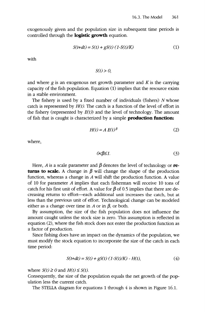
S(t+dtJ =S(t) + gS(t) (l-S(t)/KJ
(1)
with
S(t) > 0,
and where g is an exogenous net growth parameter and K is the carrying
capacity of the fish population. Equation (1) implies that the resource exists
in a stable environment.
The fishery is used by a fixed number of individuals (fishers) N whose
catch is represented by Htt). The catch is a function of the level of effort in
the fishery (represented by E(t)) and the level of technology. The amount
of fish that is caught is characterized by a simple production function:
H(t) =A E(t)(3
(2)
where,
Here, A is a scale parameter and {3 denotes the level of technology or returns to scale. A change in {3 will change the shape of the production
function, whereas a change in A will shift the production function . A value
of 10 for parameter A implies that each fisherman will receive 10 tons of
catch for his first unit of effort. A value for {3 of 0.5 implies that there are decreasing returns to effort---each additional unit increases the catch, but at
less than the previous unit of effort. Technological change can be modeled
either as a change over time in A or in {3, or both.
By assumpt ion, the size of the fish population doe s not influence the
amount caught unless the stock size is zero. This assumption is reflected in
equation (2), where the fish stock does not enter the production function as
a factor of production.
Since fishing does have an impact on the dynamics of the population, we
must modify the stock equation to incorporate the size of the catch in each
time period :
S(t+dtJ =S(t) + gS(t) (l -S(t)/KJ - Hit),
where S(t) 0 and H(t) s sai
(4)
Consequently, the size of the population equals the net growth of the population less the current catch.
The STELLA diagram for equations 1 through 4 is shown in Figure 16.1.
361
exogenously given and the population size in subsequent time periods is
controlled through the logistic growth equation.
S(t+dtJ =S(t) + gS(t) (l-S(t)/KJ
(1)
with
S(t) > 0,
and where g is an exogenous net growth parameter and K is the carrying
capacity of the fish population. Equation (1) implies that the resource exists
in a stable environment.
The fishery is used by a fixed number of individuals (fishers) N whose
catch is represented by Htt). The catch is a function of the level of effort in
the fishery (represented by E(t)) and the level of technology. The amount
of fish that is caught is characterized by a simple production function:
H(t) =A E(t)(3
(2)
where,
Here, A is a scale parameter and {3 denotes the level of technology or returns to scale. A change in {3 will change the shape of the production
function, whereas a change in A will shift the production function . A value
of 10 for parameter A implies that each fisherman will receive 10 tons of
catch for his first unit of effort. A value for {3 of 0.5 implies that there are decreasing returns to effort---each additional unit increases the catch, but at
less than the previous unit of effort. Technological change can be modeled
either as a change over time in A or in {3, or both.
By assumpt ion, the size of the fish population doe s not influence the
amount caught unless the stock size is zero. This assumption is reflected in
equation (2), where the fish stock does not enter the production function as
a factor of production.
Since fishing does have an impact on the dynamics of the population, we
must modify the stock equation to incorporate the size of the catch in each
time period :
S(t+dtJ =S(t) + gS(t) (l -S(t)/KJ - Hit),
where S(t) 0 and H(t) s sai
(4)
Consequently, the size of the population equals the net growth of the population less the current catch.
The STELLA diagram for equations 1 through 4 is shown in Figure 16.1.