

15.2. The Model
345
JCOD
C0==<
MOVE IN
MOVE RATE
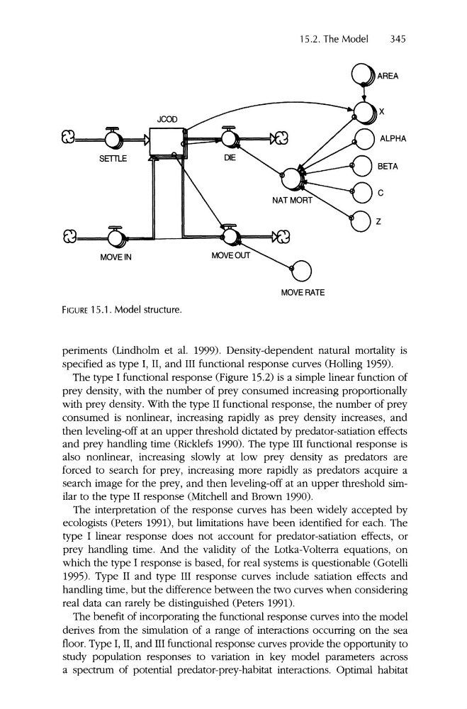
FIGURE 15.1. Model structure.
periments (Lindholm et al. 1999). Density-dependent natural mortality is
specified as type I, II, and III functional response curves (Holling 1959).
The type I functional response (Figure 15.2) is a simple linear function of
prey density, with the number of prey consumed increasing proportionally
with prey density . With the type II functional response, the number of prey
consumed is nonlinear, increasing rapidly as prey density increases, and
then leveling-off at an upper threshold dictated by predator-satiation effects
and prey handling time (Ricklefs 1990). The type III functional response is
also nonlinear, increasing slowly at low prey density as predators are
forced to search for prey, increasing more rapidly as predators acquire a
search image for the prey , and then leveling-off at an upper threshold similar to the type II response (Mitchell and Brown 1990).
The interpretation of the response curves has been widely accepted by
ecologists (Peters 1991), but limitations have been identified for each. The
type I linear response does not account for predator-satiation effects, or
prey handling time. And the validity of the Lotka-Volterra equations, on
which the type I response is based, for real systems is questionable (Gotelli
1995). Type II and type III response curves include satiation effects and
handling time, but the difference between the two curves when considering
real data can rarely be distinguished (Peters 1991).
The benefit of incorporating the functional response curves into the model
derives from the simulation of a range of interactions occurring on the sea
floor. Type I, II, and III functional response curves provide the opportunity to
study population responses to variation in key model parameters across
a spectrum of potential predator-prey-habitat interactions. Optimal habitat
345
JCOD
C0==<
MOVE IN
MOVE RATE
FIGURE 15.1. Model structure.
periments (Lindholm et al. 1999). Density-dependent natural mortality is
specified as type I, II, and III functional response curves (Holling 1959).
The type I functional response (Figure 15.2) is a simple linear function of
prey density, with the number of prey consumed increasing proportionally
with prey density . With the type II functional response, the number of prey
consumed is nonlinear, increasing rapidly as prey density increases, and
then leveling-off at an upper threshold dictated by predator-satiation effects
and prey handling time (Ricklefs 1990). The type III functional response is
also nonlinear, increasing slowly at low prey density as predators are
forced to search for prey, increasing more rapidly as predators acquire a
search image for the prey , and then leveling-off at an upper threshold similar to the type II response (Mitchell and Brown 1990).
The interpretation of the response curves has been widely accepted by
ecologists (Peters 1991), but limitations have been identified for each. The
type I linear response does not account for predator-satiation effects, or
prey handling time. And the validity of the Lotka-Volterra equations, on
which the type I response is based, for real systems is questionable (Gotelli
1995). Type II and type III response curves include satiation effects and
handling time, but the difference between the two curves when considering
real data can rarely be distinguished (Peters 1991).
The benefit of incorporating the functional response curves into the model
derives from the simulation of a range of interactions occurring on the sea
floor. Type I, II, and III functional response curves provide the opportunity to
study population responses to variation in key model parameters across
a spectrum of potential predator-prey-habitat interactions. Optimal habitat