

6.1. Basic Model
99
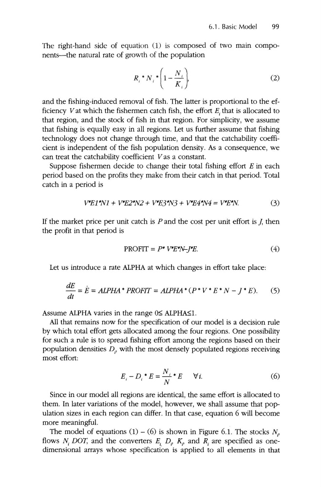
The right-hand side of equation (1) is composed of two main components-the natural rate of growth of the population
R' N'
I
I
(1- K . '
N t)
(2)
I
and the fishing-induced removal of fish. The latter is proportional to the efficiency Vat which the fishermen catch fish, the effort E, that is allocated to
that region, and the stock of fish in that region. For simplicity, we assume
that fishing is equally easy in all regions . Let us further assume that fishing
technology does not change through time, and that the catchability coefficient is independent of the fish population density. As a consequence, we
can treat the catchability coefficient Vas a constant.
Suppose fishermen decide to change their total fishing effort E in each
period based on the profits they make from their catch in that period. Total
catch in a period is
V*El *Nl + V*E2*N2 + V*E3*N3 + V*E4*N4 = V*EW
(3)
If the market price per unit catch is P and the cost per unit effort is], then
the profit in that period is
PROFIT = p* V*EW-J*E.
(4)
Let us introduce a rate ALPHA at which changes in effort take place:
dE =E= ALPHA • PROFIT = ALPHA • (P' V' E • N - ] • E) .
dt
Assume ALPHA varies in the range 0:5 ALPHA:51 .
(5)
All that remains now for the specification of our model is a decision rule
by which total effort gets allocated among the four regions . One possibility
for such a rule is to spread fishing effort among the regions based on their
population densities D i
, with the most densely populated regions receiving
most effort:
E - D • E = N i ' E
I
I
N
Vi.
(6)
Since in our model all regions are identical, the same effort is allocated to
them. In later variations of the model, however, we shall assume that population sizes in each region can differ. In that case, equation 6 will become
more meaningful.
The model of equations (1) - (6) is shown in Figure 6.1. The stocks
flows N DOT, and the converters E. D, K, and R. are specified as oner
I,
, t
,
dimensional arrays whose specification is applied to all elements in that
99
The right-hand side of equation (1) is composed of two main components-the natural rate of growth of the population
R' N'
I
I
(1- K . '
N t)
(2)
I
and the fishing-induced removal of fish. The latter is proportional to the efficiency Vat which the fishermen catch fish, the effort E, that is allocated to
that region, and the stock of fish in that region. For simplicity, we assume
that fishing is equally easy in all regions . Let us further assume that fishing
technology does not change through time, and that the catchability coefficient is independent of the fish population density. As a consequence, we
can treat the catchability coefficient Vas a constant.
Suppose fishermen decide to change their total fishing effort E in each
period based on the profits they make from their catch in that period. Total
catch in a period is
V*El *Nl + V*E2*N2 + V*E3*N3 + V*E4*N4 = V*EW
(3)
If the market price per unit catch is P and the cost per unit effort is], then
the profit in that period is
PROFIT = p* V*EW-J*E.
(4)
Let us introduce a rate ALPHA at which changes in effort take place:
dE =E= ALPHA • PROFIT = ALPHA • (P' V' E • N - ] • E) .
dt
Assume ALPHA varies in the range 0:5 ALPHA:51 .
(5)
All that remains now for the specification of our model is a decision rule
by which total effort gets allocated among the four regions . One possibility
for such a rule is to spread fishing effort among the regions based on their
population densities D i
, with the most densely populated regions receiving
most effort:
E - D • E = N i ' E
I
I
N
Vi.
(6)
Since in our model all regions are identical, the same effort is allocated to
them. In later variations of the model, however, we shall assume that population sizes in each region can differ. In that case, equation 6 will become
more meaningful.
The model of equations (1) - (6) is shown in Figure 6.1. The stocks
flows N DOT, and the converters E. D, K, and R. are specified as oner
I,
, t
,
dimensional arrays whose specification is applied to all elements in that