

100
6. Spatial Fisheries Model
Ri
Ni
Ni DOT
V
V
J
FIGURE 6.1
array. Run the model over 1000 periods with a DT= .125. The results in Figures 6.2 and 6.3 are for R t =.6 Ci =1, .. . 4), P =2.9,]=.22 and ALPHA =.6.
Changes in population sizes follow a damped oscillation, i.e. the peaks
to which population size N rises become lower for later periods. That behavior is closely matched by changes in total effort E. Since our four regions are identical, the populations in each region and the effort allocated
to each region show the same behavior (Figure 6.3).
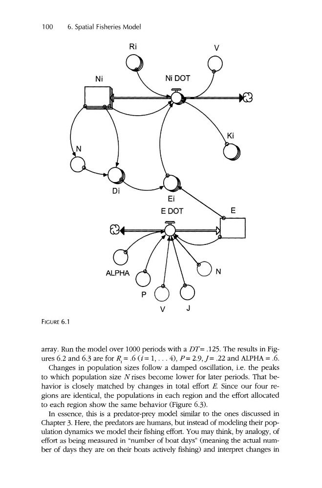
In essence, this is a predator-prey model similar to the ones discussed in
Chapter 3. Here, the predators are humans, but instead of modeling their population dynamics we model their fishing effort. You may think, by analogy, of
effort as being measured in "number of boat days" (meaning the actual number of days they are on their boats actively fishing) and interpret changes in
6. Spatial Fisheries Model
Ri
Ni
Ni DOT
V
V
J
FIGURE 6.1
array. Run the model over 1000 periods with a DT= .125. The results in Figures 6.2 and 6.3 are for R t =.6 Ci =1, .. . 4), P =2.9,]=.22 and ALPHA =.6.
Changes in population sizes follow a damped oscillation, i.e. the peaks
to which population size N rises become lower for later periods. That behavior is closely matched by changes in total effort E. Since our four regions are identical, the populations in each region and the effort allocated
to each region show the same behavior (Figure 6.3).
In essence, this is a predator-prey model similar to the ones discussed in
Chapter 3. Here, the predators are humans, but instead of modeling their population dynamics we model their fishing effort. You may think, by analogy, of
effort as being measured in "number of boat days" (meaning the actual number of days they are on their boats actively fishing) and interpret changes in