

368
w.w.L. Au
(A)
r III SL = 209 dB
~I.s
w
c
~ 0.8
~
:J
ll. 0.6
~
w 0.4
>
3 w
D::
0
w
c
~ 0.8
~
:J
ll. 0.6
~
w 0.4
>
3 w D::
50
100
150
200
FREQUENCY (KHZ)
(B)
100 /15
SL = 205 dB
SL = 214dB
SL = 202 dB
I
--V~----II
o
-"-"-""\./..'.._.._.._.._.._.._.._..
S.D. BAY
SL = 202 dB
~
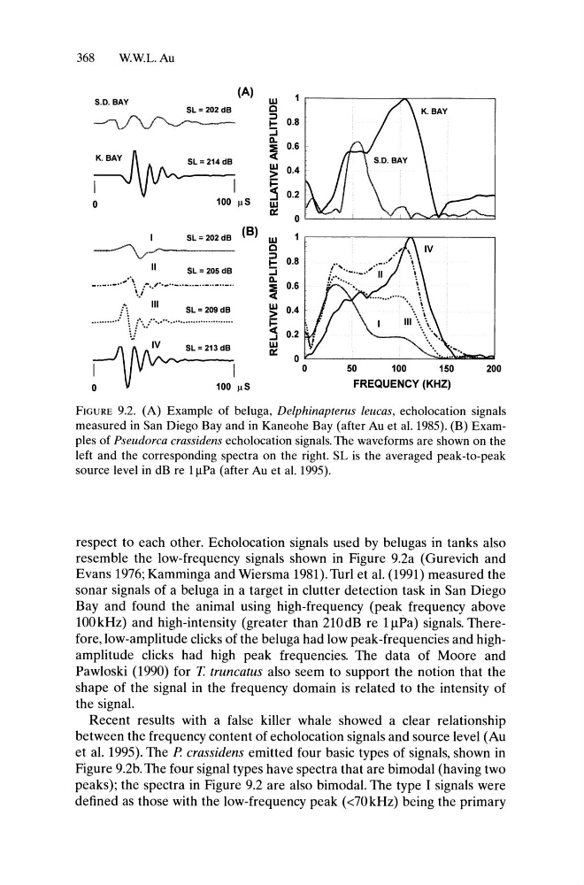
FIGURE 9.2. (A) Example of beluga, Delphinapterus leucas, echolocation signals
measured in San Diego Bay and in Kaneohe Bay (after Au et al. 1985). (B) Examples of Pseudorca crassidens echolocation signals. The waveforms are shown on the
left and the corresponding spectra on the right. SL is the averaged peak-to-peak
source level in dB re 11lPa (after Au et al. 1995).
respect to each other. Echolocation signals used by belugas in tanks also
resemble the low-frequency signals shown in Figure 9.2a (Gurevich and
Evans 1976; Kamminga and Wiersma 1981). Turl et al. (1991) measured the
sonar signals of a beluga in a target in clutter detection task in San Diego
Bay and found the animal using high-frequency (peak frequency above
100kHz) and high-intensity (greater than 210dB re 11lPa) signals. Therefore, low-amplitude clicks of the beluga had low peak-frequencies and highamplitude clicks had high peak frequencies. The data of Moore and
Pawloski (1990) for T. truncatus also seem to support the notion that the
shape of the signal in the frequency domain is related to the intensity of
the signal.
Recent results with a false killer whale showed a clear relationship
between the frequency content of echolocation signals and source level (Au
et al. 1995). The P crassidens emitted four basic types of signals, shown in
Figure 9.2b. The four signal types have spectra that are bimodal (having two
peaks); the spectra in Figure 9.2 are also bimodal. The type I signals were
defined as those with the low-frequency peak «70kHz) being the primary
w.w.L. Au
(A)
r III SL = 209 dB
~I.s
w
c
~ 0.8
~
:J
ll. 0.6
~
w 0.4
>
3 w
D::
0
w
c
~ 0.8
~
:J
ll. 0.6
~
w 0.4
>
3 w D::
50
100
150
200
FREQUENCY (KHZ)
(B)
100 /15
SL = 205 dB
SL = 214dB
SL = 202 dB
I
--V~----II
o
-"-"-""\./..'.._.._.._.._.._.._.._..
S.D. BAY
SL = 202 dB
~
FIGURE 9.2. (A) Example of beluga, Delphinapterus leucas, echolocation signals
measured in San Diego Bay and in Kaneohe Bay (after Au et al. 1985). (B) Examples of Pseudorca crassidens echolocation signals. The waveforms are shown on the
left and the corresponding spectra on the right. SL is the averaged peak-to-peak
source level in dB re 11lPa (after Au et al. 1995).
respect to each other. Echolocation signals used by belugas in tanks also
resemble the low-frequency signals shown in Figure 9.2a (Gurevich and
Evans 1976; Kamminga and Wiersma 1981). Turl et al. (1991) measured the
sonar signals of a beluga in a target in clutter detection task in San Diego
Bay and found the animal using high-frequency (peak frequency above
100kHz) and high-intensity (greater than 210dB re 11lPa) signals. Therefore, low-amplitude clicks of the beluga had low peak-frequencies and highamplitude clicks had high peak frequencies. The data of Moore and
Pawloski (1990) for T. truncatus also seem to support the notion that the
shape of the signal in the frequency domain is related to the intensity of
the signal.
Recent results with a false killer whale showed a clear relationship
between the frequency content of echolocation signals and source level (Au
et al. 1995). The P crassidens emitted four basic types of signals, shown in
Figure 9.2b. The four signal types have spectra that are bimodal (having two
peaks); the spectra in Figure 9.2 are also bimodal. The type I signals were
defined as those with the low-frequency peak «70kHz) being the primary