

8 Defining a Sampling Strategy for Okadaic Acid (OA) Toxins in Shellfish. . .
97
Table 8.2 An example of calculation of the probabilities of acceptance
c (g/kg) S
2
s
S
2
s for pools for a pool
size of 30 shellfish
mu
sigma
Probability
of acceptance
10
7.35211953 0.24507065
2.301361234 0.04947432 1
20
10.0340935
0.334469783
2.99531436
0.02891064 1
30
13.6944226
0.456480755
3.40094385
0.02251826 1
There is between mussels variability, even for mussels taken at the same sampling
point and at the same time. This variability probably stems from food access
variability and variability of response to the toxins. As regards food access, the
variability is primarily due to the fact that toxic dinoflagellates are drifted by the
currents. Moreover, accumulation and elimination rates of DSP toxins vary within a
shellfish species after a contamination event (Duinker et al. 2007). After ingestion,
a fraction of the toxins may be transformed by acylation. Acylation has been
demonstrated in bivalves by Suzuki and Mitsuya (Suzuki et al. 1999; Suzuki and
Mitsuya 2001).
Probabilities of Acceptance
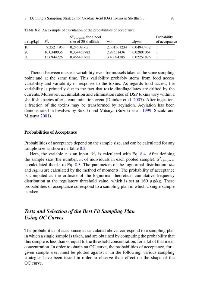
Probabilities of acceptance depend on the sample size, and can be calculated for any
sample size as shown in Table 8.2.
Here, the variable c is an input. S
2
s is calculated with Eq. 8.4. After defining
the sample size (the number, n, of individuals in each pooled sample), S
2
s for pools
is calculated thanks to Eq. 8.3. The parameters of the lognormal distribution: mu
and sigma are calculated by the method of moments. The probability of acceptance
is computed as the ordinate of the lognormal theoretical cumulative frequency
distribution at the regulatory threshold value, which is set at 160 g/kg. These
probabilities of acceptance correspond to a sampling plan in which a single sample
is taken.
Tests and Selection of the Best Fit Sampling Plan
Using OC Curves
The probabilities of acceptance as calculated above, correspond to a sampling plan
in which a single sample is taken, and are obtained by computing the probability that
this sample is less than or equal to the threshold concentration, for a lot of that mean
concentration. In order to obtain an OC curve, the probabilities of acceptance, for a
given sample size, must be plotted against c. In the following, various sampling
strategies have been tested in order to observe their effect on the shape of the
OC curve.
97
Table 8.2 An example of calculation of the probabilities of acceptance
c (g/kg) S
2
s
S
2
s for pools for a pool
size of 30 shellfish
mu
sigma
Probability
of acceptance
10
7.35211953 0.24507065
2.301361234 0.04947432 1
20
10.0340935
0.334469783
2.99531436
0.02891064 1
30
13.6944226
0.456480755
3.40094385
0.02251826 1
There is between mussels variability, even for mussels taken at the same sampling
point and at the same time. This variability probably stems from food access
variability and variability of response to the toxins. As regards food access, the
variability is primarily due to the fact that toxic dinoflagellates are drifted by the
currents. Moreover, accumulation and elimination rates of DSP toxins vary within a
shellfish species after a contamination event (Duinker et al. 2007). After ingestion,
a fraction of the toxins may be transformed by acylation. Acylation has been
demonstrated in bivalves by Suzuki and Mitsuya (Suzuki et al. 1999; Suzuki and
Mitsuya 2001).
Probabilities of Acceptance
Probabilities of acceptance depend on the sample size, and can be calculated for any
sample size as shown in Table 8.2.
Here, the variable c is an input. S
2
s is calculated with Eq. 8.4. After defining
the sample size (the number, n, of individuals in each pooled sample), S
2
s for pools
is calculated thanks to Eq. 8.3. The parameters of the lognormal distribution: mu
and sigma are calculated by the method of moments. The probability of acceptance
is computed as the ordinate of the lognormal theoretical cumulative frequency
distribution at the regulatory threshold value, which is set at 160 g/kg. These
probabilities of acceptance correspond to a sampling plan in which a single sample
is taken.
Tests and Selection of the Best Fit Sampling Plan
Using OC Curves
The probabilities of acceptance as calculated above, correspond to a sampling plan
in which a single sample is taken, and are obtained by computing the probability that
this sample is less than or equal to the threshold concentration, for a lot of that mean
concentration. In order to obtain an OC curve, the probabilities of acceptance, for a
given sample size, must be plotted against c. In the following, various sampling
strategies have been tested in order to observe their effect on the shape of the
OC curve.