

8 Defining a Sampling Strategy for Okadaic Acid (OA) Toxins in Shellfish. . .
95
Results with Interpretation
For Whitaker’s Method
Theoretical Distribution
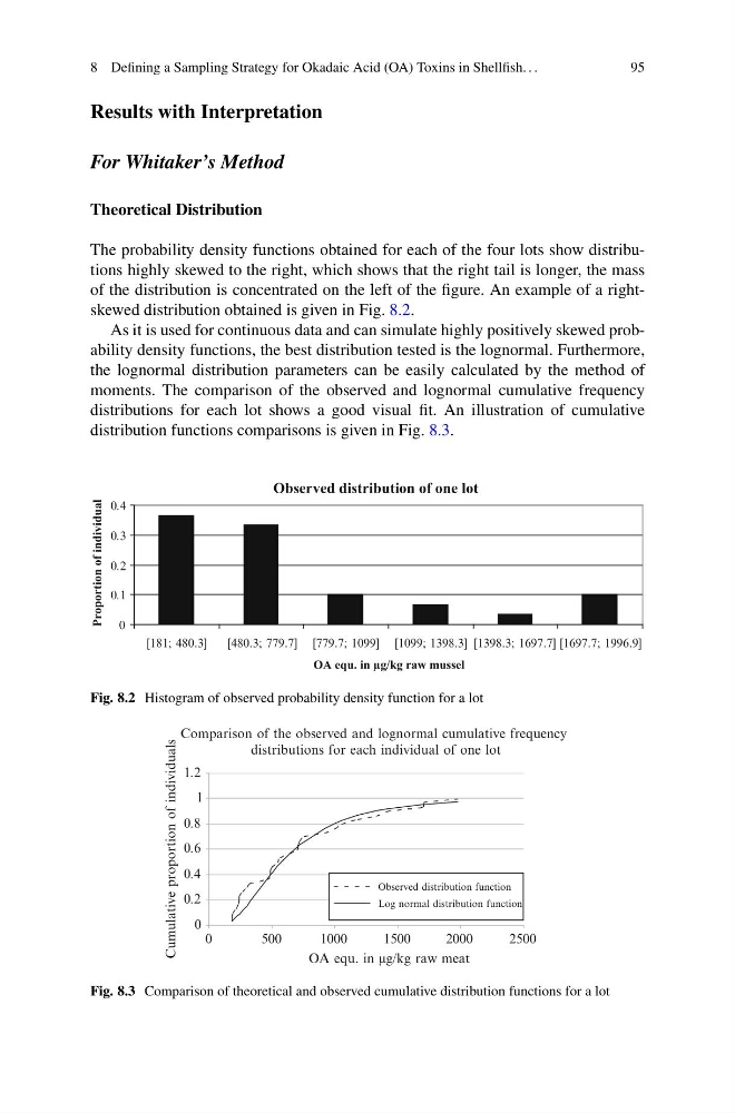
The probability density functions obtained for each of the four lots show distributions highly skewed to the right, which shows that the right tail is longer, the mass
of the distribution is concentrated on the left of the figure. An example of a rightskewed distribution obtained is given in Fig. 8.2.
As it is used for continuous data and can simulate highly positively skewed probability density functions, the best distribution tested is the lognormal. Furthermore,
the lognormal distribution parameters can be easily calculated by the method of
moments. The comparison of the observed and lognormal cumulative frequency
distributions for each lot shows a good visual fit. An illustration of cumulative
distribution functions comparisons is given in Fig. 8.3.
Observed distribution of one lot
0
0.1
0.2
0.3
0.4
[181; 480.3]
[480.3; 779.7] [779.7; 1099] [1099; 1398.3] [1398.3; 1697.7] [1697.7; 1996.9]
OA equ. in µg/kg raw mussel
Proportion of individual
Fig. 8.2 Histogram of observed probability density function for a lot
Comparison of the observed and lognormal cumulative frequency
distributions for each individual of one lot
0
0.2
0.4
0.6
0.8
1
1.2
0
500
1000
1500
2000
2500
OA equ. in µg/kg raw meat
Cumulative proportion of individuals
Observed distribution function
Log normal distribution function
Fig. 8.3 Comparison of theoretical and observed cumulative distribution functions for a lot
95
Results with Interpretation
For Whitaker’s Method
Theoretical Distribution
The probability density functions obtained for each of the four lots show distributions highly skewed to the right, which shows that the right tail is longer, the mass
of the distribution is concentrated on the left of the figure. An example of a rightskewed distribution obtained is given in Fig. 8.2.
As it is used for continuous data and can simulate highly positively skewed probability density functions, the best distribution tested is the lognormal. Furthermore,
the lognormal distribution parameters can be easily calculated by the method of
moments. The comparison of the observed and lognormal cumulative frequency
distributions for each lot shows a good visual fit. An illustration of cumulative
distribution functions comparisons is given in Fig. 8.3.
Observed distribution of one lot
0
0.1
0.2
0.3
0.4
[181; 480.3]
[480.3; 779.7] [779.7; 1099] [1099; 1398.3] [1398.3; 1697.7] [1697.7; 1996.9]
OA equ. in µg/kg raw mussel
Proportion of individual
Fig. 8.2 Histogram of observed probability density function for a lot
Comparison of the observed and lognormal cumulative frequency
distributions for each individual of one lot
0
0.2
0.4
0.6
0.8
1
1.2
0
500
1000
1500
2000
2500
OA equ. in µg/kg raw meat
Cumulative proportion of individuals
Observed distribution function
Log normal distribution function
Fig. 8.3 Comparison of theoretical and observed cumulative distribution functions for a lot