

262
Appendices
of each time step, but at any time over the whole solution interval with very
little computational overhead. According to Hairer et a1. (1987), a maximum local error of 10"' (which was used in all simulations) should give a
global truncation error on the order 10-' for reasonably smooth problems.
Numerical Solution for the Intrinsic Rate of Increase. The integral term in
Eq. (4.32) was computed by an adaptive numerical integration method
(Press et al. 1986) using 250 days as the upper limit (well above the maximum longevity in any Daphnia species). The implicit equation for A. [Eq.
(4.32)] was solved numerically using a derivative-free bracketing and
bisection method (Press et al. 1986), where the interval bracketing the root
is halved in each iteration. From an initial interval (-1, 1), the root will be
known within a precision of 2. 10-' after 16 iterations.
Peak Detection and Periodic Solutions. The differential equation solver
incorporated a simple peak detection mechanism based on the following
algorithm: if the derivative of a state variable was found to change sign
from positive in one computed solution to negative in the next, then the
state variable must have had a local maximum (with a corresponding zero
time derivative) within the last time step. The location of the peak was
found by solving the cubic equation resulting from taking the derivative of
the interpolating polynomial, and choosing the root located within the last
time step that also had a negative second derivative. Although the quartic
interpolation polynomial could in principle have two maxima within the
last time step, this condition was never flagged in all the simulations performed in this work.
Period Averages of State Variables. Periodic solutions were investigated by
monitoring the peaks of a single state variable (usually the zooplankton
biomass, Z, which had the sharpest peaks). Periods of individual cycles
could then be computed as the successive differences between the recorded
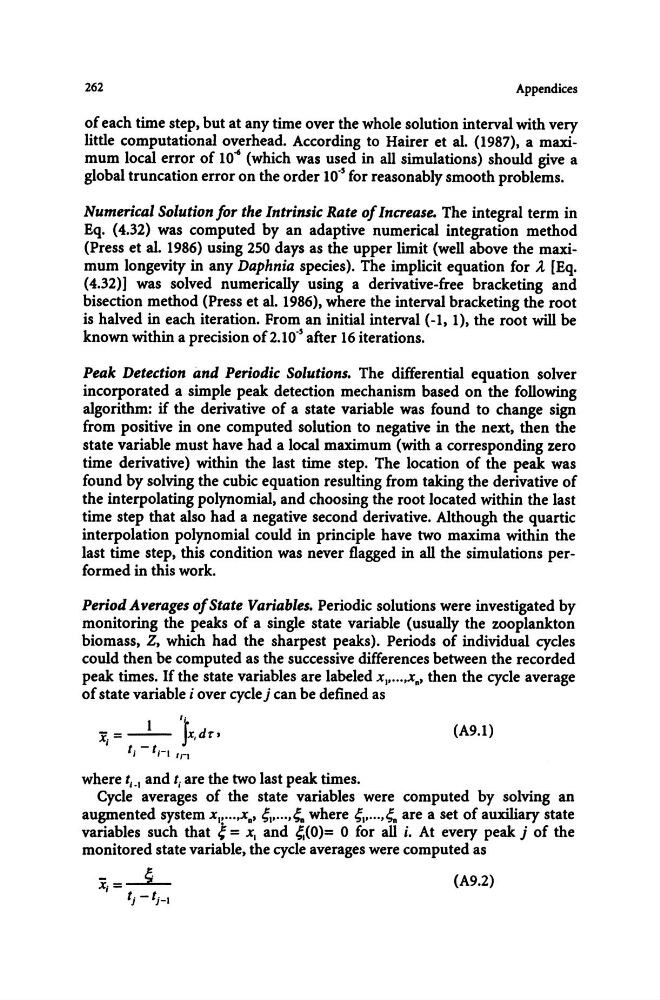
peak times. If the state variables are labeled X.""'X.' then the cycle average
of state variable i over cycle j can be defined as
1
';
X. = - - Jx,dr,
,
I· - 1'-1
I
I
Irl
where t l _. and ti are the two last peak times.
(A9.1)
Cycle averages of the state variables were computed by solving an
augmented system X"""X.' ;., .•. ,;. where ;1" .. ,;. are a set of auxiliary state
variables such that ~ = XI and ~(O)= 0 for all i. At every peak j of the
monitored state variable, the cycle averages were computed as
XI = - L
(A9.2)
tj - t j _.
Appendices
of each time step, but at any time over the whole solution interval with very
little computational overhead. According to Hairer et a1. (1987), a maximum local error of 10"' (which was used in all simulations) should give a
global truncation error on the order 10-' for reasonably smooth problems.
Numerical Solution for the Intrinsic Rate of Increase. The integral term in
Eq. (4.32) was computed by an adaptive numerical integration method
(Press et al. 1986) using 250 days as the upper limit (well above the maximum longevity in any Daphnia species). The implicit equation for A. [Eq.
(4.32)] was solved numerically using a derivative-free bracketing and
bisection method (Press et al. 1986), where the interval bracketing the root
is halved in each iteration. From an initial interval (-1, 1), the root will be
known within a precision of 2. 10-' after 16 iterations.
Peak Detection and Periodic Solutions. The differential equation solver
incorporated a simple peak detection mechanism based on the following
algorithm: if the derivative of a state variable was found to change sign
from positive in one computed solution to negative in the next, then the
state variable must have had a local maximum (with a corresponding zero
time derivative) within the last time step. The location of the peak was
found by solving the cubic equation resulting from taking the derivative of
the interpolating polynomial, and choosing the root located within the last
time step that also had a negative second derivative. Although the quartic
interpolation polynomial could in principle have two maxima within the
last time step, this condition was never flagged in all the simulations performed in this work.
Period Averages of State Variables. Periodic solutions were investigated by
monitoring the peaks of a single state variable (usually the zooplankton
biomass, Z, which had the sharpest peaks). Periods of individual cycles
could then be computed as the successive differences between the recorded
peak times. If the state variables are labeled X.""'X.' then the cycle average
of state variable i over cycle j can be defined as
1
';
X. = - - Jx,dr,
,
I· - 1'-1
I
I
Irl
where t l _. and ti are the two last peak times.
(A9.1)
Cycle averages of the state variables were computed by solving an
augmented system X"""X.' ;., .•. ,;. where ;1" .. ,;. are a set of auxiliary state
variables such that ~ = XI and ~(O)= 0 for all i. At every peak j of the
monitored state variable, the cycle averages were computed as
XI = - L
(A9.2)
tj - t j _.