

Numerical Considerations and Computational Procedures
261
will increase when either the maximum growth rate II' is reduced or when
the algal sedimentation loss rate u is increased. It should be noticed that
the persistence boundary will be more sensitive to a change in II', than to a
change of the same relative magnitude in u. Likewise, we can see from Eqs.
(A8.9), (A8.1O) that changes in the grazer growth and loss parameters (g"
and 6) will also affect the persistence boundary D'. in opposite directions;
D'. will increase when either the grazer growth rate on non-growing algae
g" is increased or when the grazer mortality loss rate 8 is decreased. The
persistence boundary D'. will be more sensitive to a change in g" than to a
change of the same relative magnitude in 8. The definition g" = g' Q'Ie
implies that an increase in g" can result from either an increase in the
maximal grazer growth rate g' or the algal P subsistence quota Q', or by a
decrease in the grazer P content e.
In Appendix A6 it was shown that it is possible to have a stationary point
where the grazer growth is limited by algal P content, but not by algal
biomass. The stationary point can exist only if the biomasses of both algae
and grazer are positive. The condition for positive grazer biomass is by Eq.
(A6.10) equivalent to requiring that the algal growth rate, which will be a
constant independent of the P loading conditions, is such that II > u + D.
Substituting the expression (A6.7) for the steady-state algal growth rate
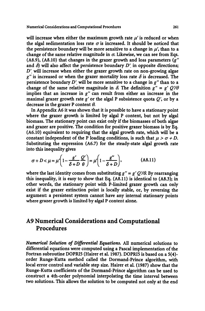
into this inequality gives
(
g' Q' ) ( g")
u+D
o+D
(A8.11)
where the last identity comes from substituting g" = g' Q'IfJ. By rearranging
this inequality, it is easy to show that Eq. (A8.11) is identical to (A8.3); in
other words, the stationary point with P-limited grazer growth can only
exist if the grazer extinction point is locally stable, or, by reversing the
argument: a persistent system cannot have any internal stationary points
where grazer growth is limited by algal P content alone.
A9 Numerical Considerations and Computational
Procedures
Numerical Solution of Differential Equations. All numerical solutions to
differential equations were computed using a Pascal implementation of the
Fortran subroutine DOPRI5 (Hairer et al. 1987). DOPRI5 is based on a 5(4)order Runge-Kutta method called the Dormand-Prince algorithm, with
local error control and variable step size. Hairer et al. (1987) show that the
Runge-Kutta coefficients of the Dormand-Prince algorithm can be used to
construct a 4th-order polynomial interpolating the time interval between
two solutions. This allows the solution to be computed not only at the end
261
will increase when either the maximum growth rate II' is reduced or when
the algal sedimentation loss rate u is increased. It should be noticed that
the persistence boundary will be more sensitive to a change in II', than to a
change of the same relative magnitude in u. Likewise, we can see from Eqs.
(A8.9), (A8.1O) that changes in the grazer growth and loss parameters (g"
and 6) will also affect the persistence boundary D'. in opposite directions;
D'. will increase when either the grazer growth rate on non-growing algae
g" is increased or when the grazer mortality loss rate 8 is decreased. The
persistence boundary D'. will be more sensitive to a change in g" than to a
change of the same relative magnitude in 8. The definition g" = g' Q'Ie
implies that an increase in g" can result from either an increase in the
maximal grazer growth rate g' or the algal P subsistence quota Q', or by a
decrease in the grazer P content e.
In Appendix A6 it was shown that it is possible to have a stationary point
where the grazer growth is limited by algal P content, but not by algal
biomass. The stationary point can exist only if the biomasses of both algae
and grazer are positive. The condition for positive grazer biomass is by Eq.
(A6.10) equivalent to requiring that the algal growth rate, which will be a
constant independent of the P loading conditions, is such that II > u + D.
Substituting the expression (A6.7) for the steady-state algal growth rate
into this inequality gives
(
g' Q' ) ( g")
u+D
o+D
(A8.11)
where the last identity comes from substituting g" = g' Q'IfJ. By rearranging
this inequality, it is easy to show that Eq. (A8.11) is identical to (A8.3); in
other words, the stationary point with P-limited grazer growth can only
exist if the grazer extinction point is locally stable, or, by reversing the
argument: a persistent system cannot have any internal stationary points
where grazer growth is limited by algal P content alone.
A9 Numerical Considerations and Computational
Procedures
Numerical Solution of Differential Equations. All numerical solutions to
differential equations were computed using a Pascal implementation of the
Fortran subroutine DOPRI5 (Hairer et al. 1987). DOPRI5 is based on a 5(4)order Runge-Kutta method called the Dormand-Prince algorithm, with
local error control and variable step size. Hairer et al. (1987) show that the
Runge-Kutta coefficients of the Dormand-Prince algorithm can be used to
construct a 4th-order polynomial interpolating the time interval between
two solutions. This allows the solution to be computed not only at the end