

Bifurcations and Long-Term Averages
141
Below the bifurcation level (denoted by p), computed solutions agree to
within numerical precision with the analytical solution at the internal focus.
The emergence of the limit cycle leads to only a modest increase in the
average zooplankton biomass compared to the asymptotic steady-state value
at the internal focus (Z1, reflecting that the zooplankton oscillations are quite
symmetrical around the asymptotic steady-state value (Fig. 5.9). On the other
hand, traversing the bifurcation level creates a dramatic jump discontinuity
in the average phytoplankton biomass, which starts to increase almost
linearly with the input P concentration when P L > p· L • This can be explained
by looking at the time course of the limit cycle (Fig. 5.9), which shows that the
maxima and minima of the phytoplankton oscillation are located very
asymmetrically with respect to the asymptotic steady-state value, leading to a
cycle average that is displaced far above the internal equilibrium.
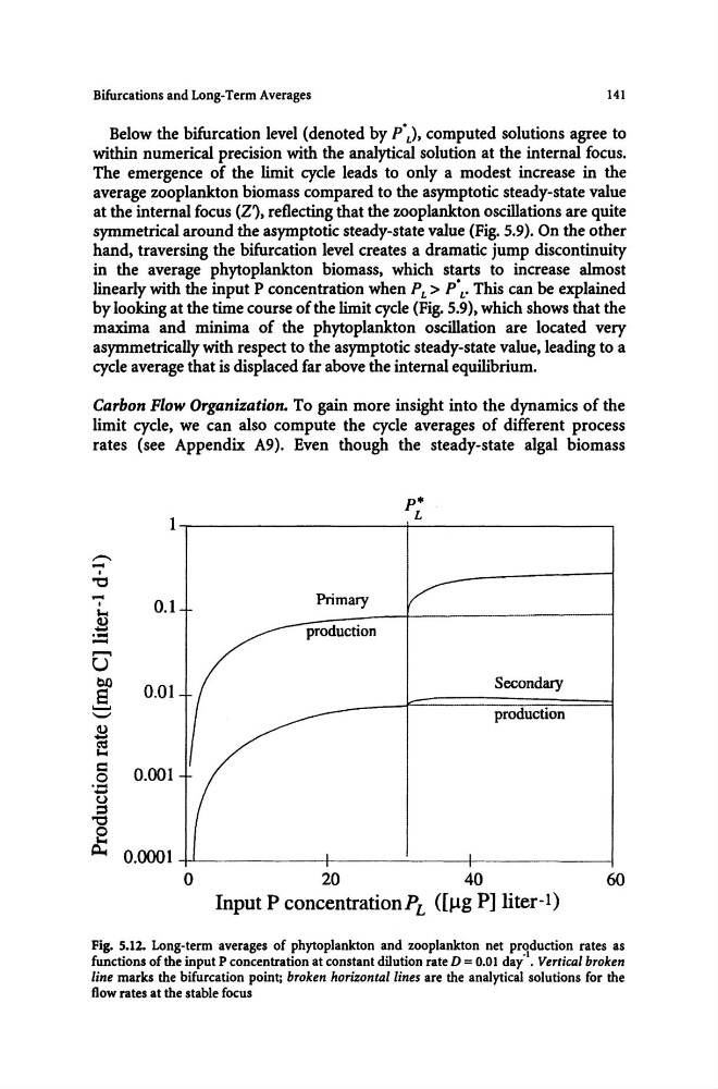
Carbon Flow Organization. To gain more insight into the dynamics of the
limit cycle, we can also compute the cycle averages of different process
rates (see Appendix A9). Even though the steady-state algal biomass
-
I
"0
-
I
B
....
- ......
U
g
'-'
~
e
c
o
.... ...
.g
e
~
p.
L
1~-------------------r-----------------.
Primary
0.1
_-----t--------0.01
Secondary
production
0.001
O.OOOl~---------+_---------r_--------~
o
w
~
~
Input P concentrationP L ([J.1g P] liter-I)
Fig. S.I2. Long-term averages of phytoplankton and zooplankton net production rates as
functions of the input P concentration at constant dilution rate D = 0.01 day·l. Vertical broken
line marks the bifurcation point; broken horizontal lines are the analytical solutions for the
flow rates at the stable focus
141
Below the bifurcation level (denoted by p), computed solutions agree to
within numerical precision with the analytical solution at the internal focus.
The emergence of the limit cycle leads to only a modest increase in the
average zooplankton biomass compared to the asymptotic steady-state value
at the internal focus (Z1, reflecting that the zooplankton oscillations are quite
symmetrical around the asymptotic steady-state value (Fig. 5.9). On the other
hand, traversing the bifurcation level creates a dramatic jump discontinuity
in the average phytoplankton biomass, which starts to increase almost
linearly with the input P concentration when P L > p· L • This can be explained
by looking at the time course of the limit cycle (Fig. 5.9), which shows that the
maxima and minima of the phytoplankton oscillation are located very
asymmetrically with respect to the asymptotic steady-state value, leading to a
cycle average that is displaced far above the internal equilibrium.
Carbon Flow Organization. To gain more insight into the dynamics of the
limit cycle, we can also compute the cycle averages of different process
rates (see Appendix A9). Even though the steady-state algal biomass
-
I
"0
-
I
B
....
- ......
U
g
'-'
~
e
c
o
.... ...
.g
e
~
p.
L
1~-------------------r-----------------.
Primary
0.1
_-----t--------0.01
Secondary
production
0.001
O.OOOl~---------+_---------r_--------~
o
w
~
~
Input P concentrationP L ([J.1g P] liter-I)
Fig. S.I2. Long-term averages of phytoplankton and zooplankton net production rates as
functions of the input P concentration at constant dilution rate D = 0.01 day·l. Vertical broken
line marks the bifurcation point; broken horizontal lines are the analytical solutions for the
flow rates at the stable focus