

3.2. MORPHOLOGICAL ANALYSIS OF A BRANCHING SPONGE
73
Set the value of the background pixels to zero
Set the value of other pixels to be the distance from the
nearest background pixel
Replace the value of each non-zero pixel with the average
value of its neighbors
for (each non-zero pixel, proceeding from the
lowest to the highest valued) {
if «(any of the pixel's non-zero neighbors are
neighbors of each other) or
(a pixel has more than three non-zero neighbors)){
set the pixel to zero
}
The remaining non -zero pixels form the digital skeleton. They may be
classified according to the number of their non-zero neighbors. Branch-tips
have only one neighbor, branches have two neighbors, and branch-vertices
have three neighbors. In order to abstract the branch structure a root
pixel is chosen at the base of each sponge's stipe and then, starting with
the root, a linked list of pixels is formed. Each member of the list contains the elements (x-position,y-position, pointer to parent
pixel, pointer to first child pixel, pointer to second
child pixel). The root pixel has a null parent, tips have two null children,
and points along the branches have one null child. The x-position and
y-position data are converted to centimeters using a scale-bar included
in each photograph, and the data is smoothed while holding the positions
of the tips, root, and vertices fixed. From this linked list the branch structure may readily be determined, and its scaling properties explored, using
Horton and fractal analyses.
3.2.2 Horton Analysis
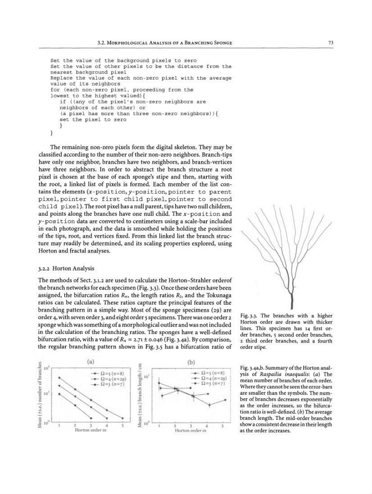
The methods of Sect. 3-1.2 are used to calculate the Horton-Strahler orderof
the branch networks for each specimen (Fig. 3.3). Once these orders have been
assigned, the bifurcation ratios R n , the length ratios R/, and the Tokunaga
ratios can be calculated . These ratios capture the principal features of the
branching pattern in a simple way. Most of the sponge specimens (29) are
order 4, with seven order 3,and eight order 5specimens. There was one order 2
sponge which was something of a morphological outlier and was not included
in the calculation of the branching ratios. The sponges have a well-defined
bifurcation ratio, with a value of R n =2.71 ± 0.046 (Fig. 3.4a). Bycomparison,
the regular branching pattern shown in Fig.3.5 has a bifurcation ratio of
Fig. 3.3. The branches with a higher
Horton order are drawn with thicker
lines. This specimen has 14 first order branches, 5 second order branches,
2 third order branches, and a fourth
order stipe.
Fig. 3-4a,b. Summary of the Horton analysis of Raspailia inaequalis: (a) The
mean number of branches of each order.
Where they cannot be seen the error-bars
are smaller than the symbols . The number of branches decreases exponentially
as the order increases , so the bifurcation ratio is well-defined. (b) The average
branch length. The mid-order branches
show a consistent decrease in their length
as the order increases.
- - Q = S (II= 8)
--.- Q = 4 (11 =29 )
Q =3 (n=7)
(b)
2
3 4
Hor ton order OJ
E
v
-
~ IO '
c
~
..c:
v
c
e
.n
.;
.,;
.!!.
c
ii 0 L-_ _~
~
- '
~ 10
Q = s (11 =8)
--.- Q =4 (11 =29)
- - Q =3 (11=7)
(a)
2 3 4
Horton order OJ
'"
-5 10 ' r - - - - - - - - - - - --.
c
~
.n
'o
...
<>
~ 10
1
§
C
73
Set the value of the background pixels to zero
Set the value of other pixels to be the distance from the
nearest background pixel
Replace the value of each non-zero pixel with the average
value of its neighbors
for (each non-zero pixel, proceeding from the
lowest to the highest valued) {
if «(any of the pixel's non-zero neighbors are
neighbors of each other) or
(a pixel has more than three non-zero neighbors)){
set the pixel to zero
}
The remaining non -zero pixels form the digital skeleton. They may be
classified according to the number of their non-zero neighbors. Branch-tips
have only one neighbor, branches have two neighbors, and branch-vertices
have three neighbors. In order to abstract the branch structure a root
pixel is chosen at the base of each sponge's stipe and then, starting with
the root, a linked list of pixels is formed. Each member of the list contains the elements (x-position,y-position, pointer to parent
pixel, pointer to first child pixel, pointer to second
child pixel). The root pixel has a null parent, tips have two null children,
and points along the branches have one null child. The x-position and
y-position data are converted to centimeters using a scale-bar included
in each photograph, and the data is smoothed while holding the positions
of the tips, root, and vertices fixed. From this linked list the branch structure may readily be determined, and its scaling properties explored, using
Horton and fractal analyses.
3.2.2 Horton Analysis
The methods of Sect. 3-1.2 are used to calculate the Horton-Strahler orderof
the branch networks for each specimen (Fig. 3.3). Once these orders have been
assigned, the bifurcation ratios R n , the length ratios R/, and the Tokunaga
ratios can be calculated . These ratios capture the principal features of the
branching pattern in a simple way. Most of the sponge specimens (29) are
order 4, with seven order 3,and eight order 5specimens. There was one order 2
sponge which was something of a morphological outlier and was not included
in the calculation of the branching ratios. The sponges have a well-defined
bifurcation ratio, with a value of R n =2.71 ± 0.046 (Fig. 3.4a). Bycomparison,
the regular branching pattern shown in Fig.3.5 has a bifurcation ratio of
Fig. 3.3. The branches with a higher
Horton order are drawn with thicker
lines. This specimen has 14 first order branches, 5 second order branches,
2 third order branches, and a fourth
order stipe.
Fig. 3-4a,b. Summary of the Horton analysis of Raspailia inaequalis: (a) The
mean number of branches of each order.
Where they cannot be seen the error-bars
are smaller than the symbols . The number of branches decreases exponentially
as the order increases , so the bifurcation ratio is well-defined. (b) The average
branch length. The mid-order branches
show a consistent decrease in their length
as the order increases.
- - Q = S (II= 8)
--.- Q = 4 (11 =29 )
Q =3 (n=7)
(b)
2
3 4
Hor ton order OJ
E
v
-
~ IO '
c
~
..c:
v
c
e
.n
.;
.,;
.!!.
c
ii 0 L-_ _~
~
- '
~ 10
Q = s (11 =8)
--.- Q =4 (11 =29)
- - Q =3 (11=7)
(a)
2 3 4
Horton order OJ
'"
-5 10 ' r - - - - - - - - - - - --.
c
~
.n
'o
...
<>
~ 10
1
§
C