

154
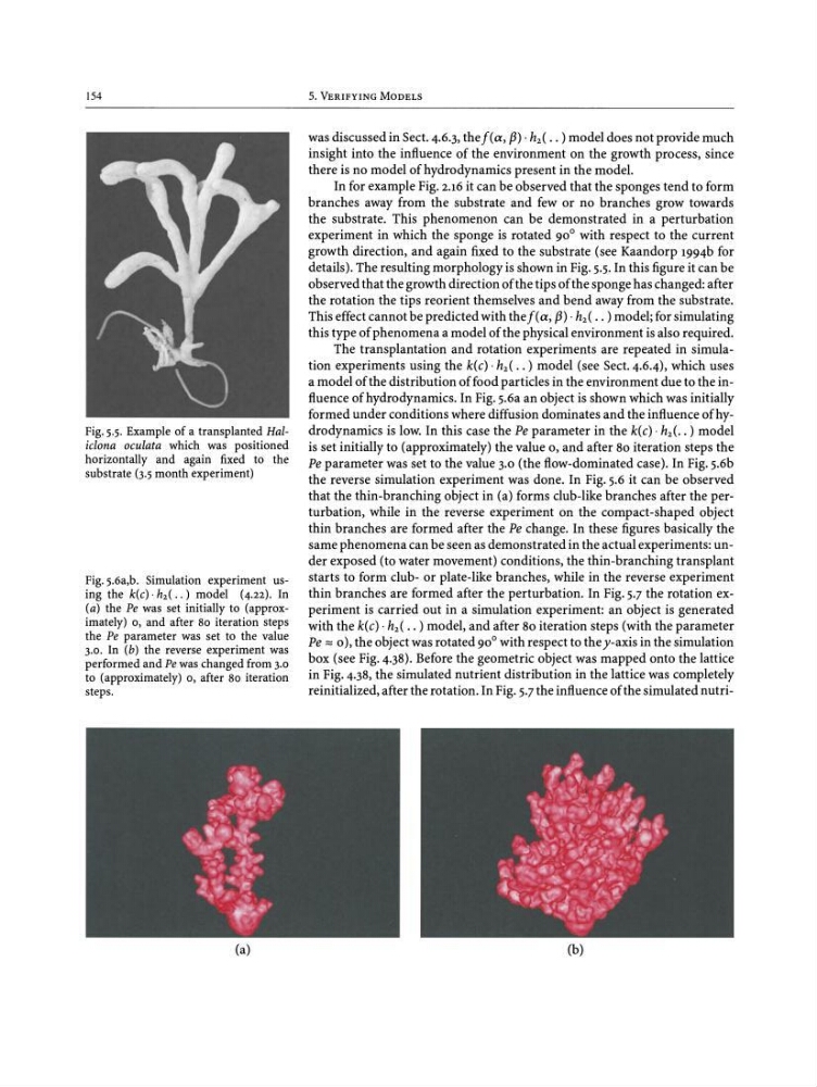
Fig. 5.5. Example of a transplanted Haliclona oculata which was positioned
horizontally and again fixed to the
substrate (3.5 month experiment)
Pig.s.ea.b. Simulation experiment using the k(c) · h 2 ( •• ) model (4.22) . In
(a) the Pe was set initially to (approximately) 0, and after 80 iteration steps
the Pe parameter was set to the value
3.0. In (b) the reverse experiment was
performed and Pewaschangedfrom 3.0
to (approximately) 0, after 80 iteration
steps.
5. VERIFYING MODELS
was discussed in Sect. 4.6.3,the f( a, 13) .h 2 ( • • ) model does not provide much
insight into the influence of the environment on the growth process, since
there is no model of hydrodynamics present in the model.
In for example Fig. 2.16 it can be observed that the sponges tend to form
branches away from the substrate and few or no branches grow towards
the substrate. This phenomenon can be demonstrated in a perturbation
experiment in which the sponge is rotated 90° with respect to the current
growth direction, and again fixed to the substrate (see Kaandorp 1994b for
details) . The resulting morphology is shown in Fig. 5.5. In this figure it can be
observed that the growth direction of the tips of the sponge has changed: after
the rotation the tips reorient themselves and bend away from the substrate.
This effect cannot be predicted with the f( a, 13) .h 2 ( •• ) model; for simulating
this type of phenomena a model of the physical environment is also required.
The transplantation and rotation experiments are repeated in simula -
tion experiments using the k(c) · h 2 ( •• ) model (see Sect. 4.6.4), which uses
a model of the distribution of food particles in the environment due to the influence of hydrodynamics. In Fig. 5.6a an object is shown which was initially
formed under conditions where diffusion dominates and the influence ofhydrodynamics is low. In this case the Pe parameter in the k(c) . h 2 ( •• ) model
is set initially to (approximately) the value 0, and after 80 iteration steps the
Pe parameter was set to the value 3.0 (the flow-dominated case). In Fig. 5.6b
the reverse simulation experiment was done. In Fig. 5.6 it can be observed
that the thin-branching object in (a) forms club-like branches after the perturbation, while in the reverse experiment on the compact-shaped object
thin branches are formed after the Pe change . In these figures basically the
same phenomena can be seen as demonstrated in the actual experiments: under exposed (to water movement) conditions, the thin-branching transplant
starts to form club- or plate-like branches, while in the reverse experiment
thin branches are formed after the perturbation. In Fig. 5.7 the rotation experiment is carried out in a simulation experiment: an object is generated
with the k(c) · h 2 ( •• ) model, and after 80 iteration steps (with the parameter
Pe ::::: 0), the object was rotated 90° with respect to the y-axis in the simulation
box (see Fig. 4.38). Before the geometric object was mapped onto the lattice
in Fig. 4.38, the simulated nutrient distribution in the lattice was completely
reinitialized, after the rotation. In Fig. 5.7 the influence of the simulated nutri(a)
(b)
Fig. 5.5. Example of a transplanted Haliclona oculata which was positioned
horizontally and again fixed to the
substrate (3.5 month experiment)
Pig.s.ea.b. Simulation experiment using the k(c) · h 2 ( •• ) model (4.22) . In
(a) the Pe was set initially to (approximately) 0, and after 80 iteration steps
the Pe parameter was set to the value
3.0. In (b) the reverse experiment was
performed and Pewaschangedfrom 3.0
to (approximately) 0, after 80 iteration
steps.
5. VERIFYING MODELS
was discussed in Sect. 4.6.3,the f( a, 13) .h 2 ( • • ) model does not provide much
insight into the influence of the environment on the growth process, since
there is no model of hydrodynamics present in the model.
In for example Fig. 2.16 it can be observed that the sponges tend to form
branches away from the substrate and few or no branches grow towards
the substrate. This phenomenon can be demonstrated in a perturbation
experiment in which the sponge is rotated 90° with respect to the current
growth direction, and again fixed to the substrate (see Kaandorp 1994b for
details) . The resulting morphology is shown in Fig. 5.5. In this figure it can be
observed that the growth direction of the tips of the sponge has changed: after
the rotation the tips reorient themselves and bend away from the substrate.
This effect cannot be predicted with the f( a, 13) .h 2 ( •• ) model; for simulating
this type of phenomena a model of the physical environment is also required.
The transplantation and rotation experiments are repeated in simula -
tion experiments using the k(c) · h 2 ( •• ) model (see Sect. 4.6.4), which uses
a model of the distribution of food particles in the environment due to the influence of hydrodynamics. In Fig. 5.6a an object is shown which was initially
formed under conditions where diffusion dominates and the influence ofhydrodynamics is low. In this case the Pe parameter in the k(c) . h 2 ( •• ) model
is set initially to (approximately) the value 0, and after 80 iteration steps the
Pe parameter was set to the value 3.0 (the flow-dominated case). In Fig. 5.6b
the reverse simulation experiment was done. In Fig. 5.6 it can be observed
that the thin-branching object in (a) forms club-like branches after the perturbation, while in the reverse experiment on the compact-shaped object
thin branches are formed after the Pe change . In these figures basically the
same phenomena can be seen as demonstrated in the actual experiments: under exposed (to water movement) conditions, the thin-branching transplant
starts to form club- or plate-like branches, while in the reverse experiment
thin branches are formed after the perturbation. In Fig. 5.7 the rotation experiment is carried out in a simulation experiment: an object is generated
with the k(c) · h 2 ( •• ) model, and after 80 iteration steps (with the parameter
Pe ::::: 0), the object was rotated 90° with respect to the y-axis in the simulation
box (see Fig. 4.38). Before the geometric object was mapped onto the lattice
in Fig. 4.38, the simulated nutrient distribution in the lattice was completely
reinitialized, after the rotation. In Fig. 5.7 the influence of the simulated nutri(a)
(b)