

4.6. ACCRETIVE GROWTH
(rest_term =0.0) or hemispherical objects (restterm = 0.3), as shown in
Fig. 4.46. With the amount of contact with the environment component, this
model produces highly complex branching patterns (see Fig. 4.47); in this
case it is also necessary to take the effects of self-shading into account.
4.6.6 A Model of Accretive Growth Driven by Local Nutrient Availability
and Regulated by a Growth-Suppressing Isomone
In the final model we have combined the model described in Sect. 4.6.4, using
the growth function shown in (4.26), with a third component suppressing the
growth process. In the lattice model, independently of the nutrient, a chemical
agent (the simulated isomone) is being dispersed through both diffusion
and flow, using the computed flow velocities in the algorithm described
in Sect.4.6.4. After the (nutrient) tracer step, a second (isomone) tracer
step is done for both phases and the local mean isomone gradient iCc) =
i (i1(C) + i 2 (c)) is computed. The sources of isomone are all the voxels in the
discrete representation of the object (see Fig. 4.38) neighboring to the fluid
nodes, excluding the growing tips of the object. In the simulations only the
voxels representing the object and added delay_isomone growth steps ago
are used as source nodes. Without this restriction all surface nodes would
become source nodes and growth would be suppressed everywhere and stop
the complete growth process immediately. In all simulations this parameter
delay_isomone was set to the value 5. In the simulations it is assumed that
in every time step in the algorithm in Sect. 4.6.4 there is a constant rate
of removal decay_isomone of isomone for both phases. The isomone tracer
distribution is computed until an equilibrium is reached between the source
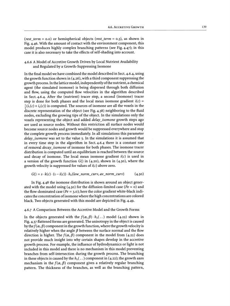
and decay of isomone. The local mean isomone gradient iCc) is used in
a version of the growth function GO in (4.20), shown in (4.30), where the
growth velocity is suppressed for values of iCc) above zero.
In Fig. 4.48 the isomone distribution is shown around an object generated with the model using (4.30) for the diffusion-limited case (Pe:::: 0) and
the flow-dominated case (Pe = 3.0); here the color gradient white-black indicates the concentration of isomone where the high concentrations are colored
black. Two objects generated with this model are depicted in Fig. 4.49.
4.6.7 A Comparison Between the Accretive Model and the Growth Forms
In the objects generated with the [La, 13) .h 2 ( •• ) model (4.22) shown in
Fig. 4.37flattened forms are generated. The anisotropy in the object is caused
by the [t«, 13) component in the growth function, where the growth velocity is
relatively higher when the angle 13 between the surface normal and the flow
direction is higher. The [t«, 13) component in the model from (4.22) does
not provide much insight into why certain shapes develop in the accretive
growth process. For example, the influence of hydrodynamics or light is not
included in this model and there is no mechanism in this model preventing
branches from self-intersection during the growth process. The branching
in these objects is caused by the h 2 ( • • ) component in (4.22); the growth axes
mechanism in the [to; 13) component gives a relatively regular branching
pattern. The thickness of the branches, as well as the branching pattern,
139
(rest_term =0.0) or hemispherical objects (restterm = 0.3), as shown in
Fig. 4.46. With the amount of contact with the environment component, this
model produces highly complex branching patterns (see Fig. 4.47); in this
case it is also necessary to take the effects of self-shading into account.
4.6.6 A Model of Accretive Growth Driven by Local Nutrient Availability
and Regulated by a Growth-Suppressing Isomone
In the final model we have combined the model described in Sect. 4.6.4, using
the growth function shown in (4.26), with a third component suppressing the
growth process. In the lattice model, independently of the nutrient, a chemical
agent (the simulated isomone) is being dispersed through both diffusion
and flow, using the computed flow velocities in the algorithm described
in Sect.4.6.4. After the (nutrient) tracer step, a second (isomone) tracer
step is done for both phases and the local mean isomone gradient iCc) =
i (i1(C) + i 2 (c)) is computed. The sources of isomone are all the voxels in the
discrete representation of the object (see Fig. 4.38) neighboring to the fluid
nodes, excluding the growing tips of the object. In the simulations only the
voxels representing the object and added delay_isomone growth steps ago
are used as source nodes. Without this restriction all surface nodes would
become source nodes and growth would be suppressed everywhere and stop
the complete growth process immediately. In all simulations this parameter
delay_isomone was set to the value 5. In the simulations it is assumed that
in every time step in the algorithm in Sect. 4.6.4 there is a constant rate
of removal decay_isomone of isomone for both phases. The isomone tracer
distribution is computed until an equilibrium is reached between the source
and decay of isomone. The local mean isomone gradient iCc) is used in
a version of the growth function GO in (4.20), shown in (4.30), where the
growth velocity is suppressed for values of iCc) above zero.
In Fig. 4.48 the isomone distribution is shown around an object generated with the model using (4.30) for the diffusion-limited case (Pe:::: 0) and
the flow-dominated case (Pe = 3.0); here the color gradient white-black indicates the concentration of isomone where the high concentrations are colored
black. Two objects generated with this model are depicted in Fig. 4.49.
4.6.7 A Comparison Between the Accretive Model and the Growth Forms
In the objects generated with the [La, 13) .h 2 ( •• ) model (4.22) shown in
Fig. 4.37flattened forms are generated. The anisotropy in the object is caused
by the [t«, 13) component in the growth function, where the growth velocity is
relatively higher when the angle 13 between the surface normal and the flow
direction is higher. The [t«, 13) component in the model from (4.22) does
not provide much insight into why certain shapes develop in the accretive
growth process. For example, the influence of hydrodynamics or light is not
included in this model and there is no mechanism in this model preventing
branches from self-intersection during the growth process. The branching
in these objects is caused by the h 2 ( • • ) component in (4.22); the growth axes
mechanism in the [to; 13) component gives a relatively regular branching
pattern. The thickness of the branches, as well as the branching pattern,
139