

4.6. ACCRETIVE GROWTH
131
(a)
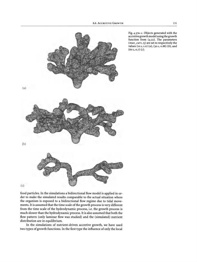
Fig.4.37a-C. Objects generated with the
accretive growthmodelusingthe growth
function from (4.22). The parameters
(max_curv, 11) are set to respectively the
values (10 S, 1.0) (a), (30 S, 0.88) (b), and
(60 S, 0.7) (c) .
(c)
food particles. In the simulations a bidirectional flow model is applied in order to make the simulated results comparable to the actual situation where
the organism is exposed to a bidirectional flow regime due to tidal movements. It is assumed that the time scale of the growth process is very different
from the time scale of the hydrodynamic process, i.e. the growth process is
much slower than the hydrodynamic process. It is also assumed that both the
flow pattern (only laminar flow was studied) and the (simulated) nutrient
distribution are in equilibrium.
In the simulations of nutrient-driven accretive growth, we have used
two types of growth functions. In the first type the influence of only the local
131
(a)
Fig.4.37a-C. Objects generated with the
accretive growthmodelusingthe growth
function from (4.22). The parameters
(max_curv, 11) are set to respectively the
values (10 S, 1.0) (a), (30 S, 0.88) (b), and
(60 S, 0.7) (c) .
(c)
food particles. In the simulations a bidirectional flow model is applied in order to make the simulated results comparable to the actual situation where
the organism is exposed to a bidirectional flow regime due to tidal movements. It is assumed that the time scale of the growth process is very different
from the time scale of the hydrodynamic process, i.e. the growth process is
much slower than the hydrodynamic process. It is also assumed that both the
flow pattern (only laminar flow was studied) and the (simulated) nutrient
distribution are in equilibrium.
In the simulations of nutrient-driven accretive growth, we have used
two types of growth functions. In the first type the influence of only the local