

130
4 . SIMULATING GROWTH AND FORM
4.6.4 A Model of Accretive Growth Driven by the Local Amount
of Available Nutrient and the Influence of Hydrodynamics
In this model it is assumed that the organism is using exclusively suspension
feeding as an energy source and that food particles are dispersed by the combined process of diffusion and hydrodynamics. Furthermore it is assumed
that transport of nutrients through the tissue is small or negligible and that
the local growth velocity is directly related to the local amount of absorbed
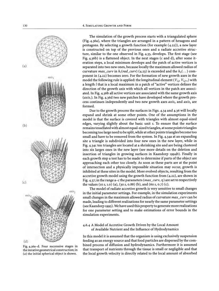
The simulation of the growth process starts with a triangulated sphere
(Fig. 4.36a), where the triangles are arranged in a pattern of hexagons and
pentagons. By selecting a growth function (for example (4.22», a new layer
is constructed on top of the previous ones and a radiate accretive structure, similar to the one observed in Fig. 4.33, develops. The first stage (see
Fig.4 .36b) is a flattened object. In the next stages (c and d), after some iteration steps, a local minimum develops and the patch of active vertices is
separated into two new ones, because locally the maximum allowed radius of
curvature max_curv in hr(rad_curv) (4.23) is exceeded and the h 2 ( • • ) component in (4.22) becomes zero. For the formation of new growth axes in the
model the following rule is applied: the longitudinal element (Vi,j' V i,j+) with
a length 1that is a local maximum in a patch of "active" vertices defines the
direction of the growth axis with which all vertices in the patch are associated. In Fig. 4.36b all active vertices are associated with the same growth axis
iaxis.) . In Fig. 4.36d two new patches have developed where the growth process continues independently and two new growth axes axis, and axis, are
formed.
Due to the growth process the surfaces in Figs. 4.34 and 4.36will locally
expand and shrink at some other points. One of the assumptions in the
model is that the surface is covered with triangles with almost equal-sized
edges, varying slightly about the basic unit 5. To ensure that the surface
remains tessellated with almost equal-sized triangles, at some points triangles
becoming too large need to be split, while at other points triangles become too
small and have to be removed from the system. In Fig. 4.34a at an expanding
site a triangle is subdivided into four new ones in the new layer, while in
Fig. 4.34C ten triangles are located at a shrinking site and are being clustered
into six larges ones in the new layer (see more details on the deletion and
insertion of triangles in growing surfaces in Kaandorp 1994b). Finally in
each growth step a test has to be made to determine if parts of the object are
approaching each other too closely. As soon as these parts are at the point
of intersection and a physically impossible situation may occur, growth is
inhibited at these sites in the model. More evolved objects, resulting from the
accretive growth model using the growth function from (4.22), are shown in
Fig. 4.37; in the range a-c the parameters (max_curv, rz) are set to respectively
the values (lOS, 1.0) (a), (305,0.88) (b), and (60S, 0.7) (c).
The model of radiate accretive growth is very sensitive to small changes
in the initial parameter settings. For example, in the simulation experiments
small changes in the maximum allowed radius of curvature max_curv can be
made, leading to different realizations for nearly the same parameter settings
(see Kaandorp 1995). Wehave used this property to generate more realizations
for one parameter setting and to make estimations of error bounds in the
simulation experiments.
(d)
Fig.4.36a-d. Four successive stages in
the iterative geometrical construction; in
(a) the initialspherical object is shown.
(b)
(a)
(c)
4 . SIMULATING GROWTH AND FORM
4.6.4 A Model of Accretive Growth Driven by the Local Amount
of Available Nutrient and the Influence of Hydrodynamics
In this model it is assumed that the organism is using exclusively suspension
feeding as an energy source and that food particles are dispersed by the combined process of diffusion and hydrodynamics. Furthermore it is assumed
that transport of nutrients through the tissue is small or negligible and that
the local growth velocity is directly related to the local amount of absorbed
The simulation of the growth process starts with a triangulated sphere
(Fig. 4.36a), where the triangles are arranged in a pattern of hexagons and
pentagons. By selecting a growth function (for example (4.22», a new layer
is constructed on top of the previous ones and a radiate accretive structure, similar to the one observed in Fig. 4.33, develops. The first stage (see
Fig.4 .36b) is a flattened object. In the next stages (c and d), after some iteration steps, a local minimum develops and the patch of active vertices is
separated into two new ones, because locally the maximum allowed radius of
curvature max_curv in hr(rad_curv) (4.23) is exceeded and the h 2 ( • • ) component in (4.22) becomes zero. For the formation of new growth axes in the
model the following rule is applied: the longitudinal element (Vi,j' V i,j+) with
a length 1that is a local maximum in a patch of "active" vertices defines the
direction of the growth axis with which all vertices in the patch are associated. In Fig. 4.36b all active vertices are associated with the same growth axis
iaxis.) . In Fig. 4.36d two new patches have developed where the growth process continues independently and two new growth axes axis, and axis, are
formed.
Due to the growth process the surfaces in Figs. 4.34 and 4.36will locally
expand and shrink at some other points. One of the assumptions in the
model is that the surface is covered with triangles with almost equal-sized
edges, varying slightly about the basic unit 5. To ensure that the surface
remains tessellated with almost equal-sized triangles, at some points triangles
becoming too large need to be split, while at other points triangles become too
small and have to be removed from the system. In Fig. 4.34a at an expanding
site a triangle is subdivided into four new ones in the new layer, while in
Fig. 4.34C ten triangles are located at a shrinking site and are being clustered
into six larges ones in the new layer (see more details on the deletion and
insertion of triangles in growing surfaces in Kaandorp 1994b). Finally in
each growth step a test has to be made to determine if parts of the object are
approaching each other too closely. As soon as these parts are at the point
of intersection and a physically impossible situation may occur, growth is
inhibited at these sites in the model. More evolved objects, resulting from the
accretive growth model using the growth function from (4.22), are shown in
Fig. 4.37; in the range a-c the parameters (max_curv, rz) are set to respectively
the values (lOS, 1.0) (a), (305,0.88) (b), and (60S, 0.7) (c).
The model of radiate accretive growth is very sensitive to small changes
in the initial parameter settings. For example, in the simulation experiments
small changes in the maximum allowed radius of curvature max_curv can be
made, leading to different realizations for nearly the same parameter settings
(see Kaandorp 1995). Wehave used this property to generate more realizations
for one parameter setting and to make estimations of error bounds in the
simulation experiments.
(d)
Fig.4.36a-d. Four successive stages in
the iterative geometrical construction; in
(a) the initialspherical object is shown.
(b)
(a)
(c)