

132
4. SIMULATING GROWTH AND FORM
availability of simulated nutrient is included in the growth function GO in
(4.2 0 ):
GO = s - k(c)
(4.25)
where k( c) is an estimate of the local nutrient gradient along the mean normal
vector on the surface of the object. In the second type of growth function:
GO = s k(c) · h 2(low_norm_curv, av_norm_curv)
(4.26)
where in the component h« ( . . ) an estimate is made of the amount of contact
with the environment.
In the simulations the diffusion coefficient D varies, and uis kept constant by adjust ing the driving force F of the system. Due to the growth of the
object the velocity in the free fluid would gradually decrease if the driving
force were not adjusted. In all simulations the corresponding Reynolds number is kept to a very low and constant value, so we are in the "creeping flow"
regime.
The simulated growth form is initialized with a spherical object (the
object shown in Fig.4.36a) which was mapped onto the 144 3 lattice and po -
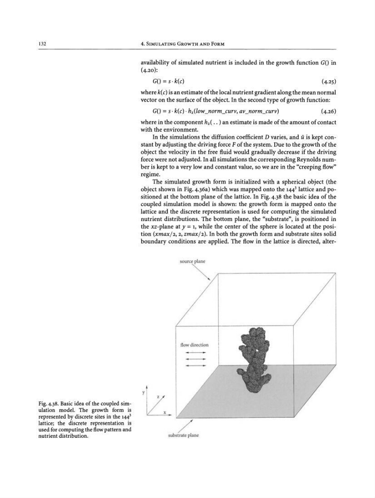
sitioned at the bottom plane of the lattice. In Fig. 4.38 the basic idea of the
coupled simulation model is shown: the growth form is mapped onto the
lattice and the discrete representation is used for computing the simulated
nutrient distributions. The bottom plane, the "substrate", is positioned in
the xz-plane at y = 1, while the center of the sphere is located at the position ixmaxfz, 2, zmax f z). In both the growth form and substrate sites solid
boundary conditions are applied. The flow in the lattice is directed, altersource plane
,
Fig. 4.38. Basic idea of the coupled simulation model. The growth form is
represented by discrete sites in the 144 3
lattice; the discrete representation is
usedforcomputing the flow pattern and
nutrient distribution.
flow d irect ion
•
Y ~
4. SIMULATING GROWTH AND FORM
availability of simulated nutrient is included in the growth function GO in
(4.2 0 ):
GO = s - k(c)
(4.25)
where k( c) is an estimate of the local nutrient gradient along the mean normal
vector on the surface of the object. In the second type of growth function:
GO = s k(c) · h 2(low_norm_curv, av_norm_curv)
(4.26)
where in the component h« ( . . ) an estimate is made of the amount of contact
with the environment.
In the simulations the diffusion coefficient D varies, and uis kept constant by adjust ing the driving force F of the system. Due to the growth of the
object the velocity in the free fluid would gradually decrease if the driving
force were not adjusted. In all simulations the corresponding Reynolds number is kept to a very low and constant value, so we are in the "creeping flow"
regime.
The simulated growth form is initialized with a spherical object (the
object shown in Fig.4.36a) which was mapped onto the 144 3 lattice and po -
sitioned at the bottom plane of the lattice. In Fig. 4.38 the basic idea of the
coupled simulation model is shown: the growth form is mapped onto the
lattice and the discrete representation is used for computing the simulated
nutrient distributions. The bottom plane, the "substrate", is positioned in
the xz-plane at y = 1, while the center of the sphere is located at the position ixmaxfz, 2, zmax f z). In both the growth form and substrate sites solid
boundary conditions are applied. The flow in the lattice is directed, altersource plane
,
Fig. 4.38. Basic idea of the coupled simulation model. The growth form is
represented by discrete sites in the 144 3
lattice; the discrete representation is
usedforcomputing the flow pattern and
nutrient distribution.
flow d irect ion
•
Y ~