

128
4. SIMULATING GROWTH AND FORM
many sponges and stony corals (see Fig. 4.33). In the basic construction, the
thickness 1of the new layer varies between a threshold value tr slightly above
zero and s the basic size of a skeleton element. In the actual organisms the
layers are connected with skeleton elements which may vary in length but
cannot become arbitrarily small, since they are made of discrete elements.
The longitudinal connection with length 1between two vertices Vij and V ij+l
in two successive growth layers j, j + 1 is made along the mean normal vector
of the triangles surrounding the vertex V ij of the previous growth layer.
In the simulations we have used various types of growth functions. The
thickness 1of a new layer is determined by a growth function GO:
1= { s - GO for GO > tr
0.0
for GO s tr
which becomes zero as soon as GOfalls below the threshold tr, i.e. no material
is being added and growth locally stops.
4.6.3 Accretive Growth Using an Approximation of Actual Deposition
Velocities and the Amount of Contact with the Environment
In the first model the distribution of growth velocities over a tip of an organism with accretive growth is approximated with a mathematical function. The
distribution was in this case obtained from sections made through growing
tips of the sponge Haliclona oculata (see for example Fig. 2.17). As discussed
in Sect. 2.2.2 this species tends to form flattened branching forms, where
most branches develop in a plane which is perpendicular to the govern ing
flow direction. Since the tips of these sponges are flattened, the deposition
of material is anisotropic. This deposition process can be approximated with
an anisotropic growth function (see Kaandorp 1995):
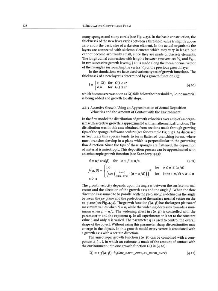
d = w] cos(f3) for 0 s f3 < ttf :
\
1.0
[ta, f3) = (cos ( ( n ! 2) . (a - TTld»)) ~
( n ! 2- n ! d )
W>2
for 0 s a s (rr /d)
for (rr /2+rr/d)
vector and the direction of the growth axis and the angle f3. When the flow
direction is assumed to be parallel with the yz-plane, f3 is defined as the angle
between the yx -plane and the projection of the surface normal vector on the
xz-plane (see Fig. 4.35). The growth functionf(a, f3) has the largest plateau of
maximum values when f3 = 0 , while the widening decreases towards a minimum when f3 =nl». The widening effect in [ta, f3) is controlled with the
parameter wand the exponent rz. In all experiments w is set to the constant
value 8 and only rz is varied. The parameter rz is used to control the overall
shape of the object. Without using this parameter sharp discontinuities may
emerge in the objects. In this growth model every vertex is associated with
a growth axis with a certain direction.
The anisotropic growth functionf(a, f3) can be combined with a component h 2 ( •• ), in which an estimate is made of the amount of contact with
the environment, into one growth function GO in (4.20):
4. SIMULATING GROWTH AND FORM
many sponges and stony corals (see Fig. 4.33). In the basic construction, the
thickness 1of the new layer varies between a threshold value tr slightly above
zero and s the basic size of a skeleton element. In the actual organisms the
layers are connected with skeleton elements which may vary in length but
cannot become arbitrarily small, since they are made of discrete elements.
The longitudinal connection with length 1between two vertices Vij and V ij+l
in two successive growth layers j, j + 1 is made along the mean normal vector
of the triangles surrounding the vertex V ij of the previous growth layer.
In the simulations we have used various types of growth functions. The
thickness 1of a new layer is determined by a growth function GO:
1= { s - GO for GO > tr
0.0
for GO s tr
which becomes zero as soon as GOfalls below the threshold tr, i.e. no material
is being added and growth locally stops.
4.6.3 Accretive Growth Using an Approximation of Actual Deposition
Velocities and the Amount of Contact with the Environment
In the first model the distribution of growth velocities over a tip of an organism with accretive growth is approximated with a mathematical function. The
distribution was in this case obtained from sections made through growing
tips of the sponge Haliclona oculata (see for example Fig. 2.17). As discussed
in Sect. 2.2.2 this species tends to form flattened branching forms, where
most branches develop in a plane which is perpendicular to the govern ing
flow direction. Since the tips of these sponges are flattened, the deposition
of material is anisotropic. This deposition process can be approximated with
an anisotropic growth function (see Kaandorp 1995):
d = w] cos(f3) for 0 s f3 < ttf :
\
1.0
[ta, f3) = (cos ( ( n ! 2) . (a - TTld»)) ~
( n ! 2- n ! d )
W>2
for 0 s a s (rr /d)
for (rr /2+rr/d)
vector and the direction of the growth axis and the angle f3. When the flow
direction is assumed to be parallel with the yz-plane, f3 is defined as the angle
between the yx -plane and the projection of the surface normal vector on the
xz-plane (see Fig. 4.35). The growth functionf(a, f3) has the largest plateau of
maximum values when f3 = 0 , while the widening decreases towards a minimum when f3 =nl». The widening effect in [ta, f3) is controlled with the
parameter wand the exponent rz. In all experiments w is set to the constant
value 8 and only rz is varied. The parameter rz is used to control the overall
shape of the object. Without using this parameter sharp discontinuities may
emerge in the objects. In this growth model every vertex is associated with
a growth axis with a certain direction.
The anisotropic growth functionf(a, f3) can be combined with a component h 2 ( •• ), in which an estimate is made of the amount of contact with
the environment, into one growth function GO in (4.20):